Logistic Regression: Classification and Probability Interpretation

1. What is Classification?

Classification is about assigning items to predefined categories. While it might seem completely different from regression, there's a strong conceptual link. Let's explore why we need a new tool for these problems and can't just use the linear regression models you've already mastered.

The following video provides an excellent introduction to classification and explains the limitations of using linear regression for this type of task.

As you saw, a straight line doesn't work well because it can predict values outside the sensible 0-to-1 range and is easily thrown off by outliers. We need a model that is specifically designed to output a value that can be interpreted as a probability—a number between 0 and 1.

2. The Core Idea: The Sigmoid Function

Logistic regression solves this problem elegantly. It starts with the same linear equation you know from linear regression:

$z={\beta }_0+{\beta }_1{x}_1+{\beta }_2{x}_2+\cdots +{\beta }_p{x}_p$

However, instead of using the output $z$ directly, it passes this value through a special function called the sigmoid (or logistic) function. This function "squashes" any real number into a value between 0 and 1.

To build a strong intuition for this process, watch the following short video.

The sigmoid function is defined by the following formula:

$p=\frac{1}{1+e^{-z}}$

Where:

• $p$ is the predicted probability of the outcome being 1.
• $e$ is Euler's number (approximately 2.718).
• $z$ is the output of our linear equation.

This mathematical transformation ensures that our model's output is always a valid probability. If the linear equation $z$ produces a large positive number, $e^{-z}$ becomes very small, and $p$ gets close to 1. If $z$ is a large negative number, $e^{-z}$ becomes very large, and $p$ gets close to 0.

3. Training a Logistic Regression Classifier in Python

Now for the practical part. Since you're already familiar with the scikit-learn API from our regression module, you'll find the process for training a logistic regression model very familiar. The steps are nearly identical: import the model, split the data, and use the .fit() method.

The codebasics video you watched earlier continues with a great hands-on coding example.

As you can see, with just a few lines of code, you have a trained classification model ready to make predictions.

4. Interpreting the Output: From Probabilities to Predictions

This is the most critical part of our lesson. How do we get from a trained model to an interpretable result? Logistic regression models in scikit-learn have two key methods for this: .predict() and .predict_proba().

• model.predict(X_test): This gives you the final classification—0 or 1. By default, it classifies an instance as '1' if the calculated probability is > 0.5, and '0' otherwise.
• model.predict_proba(X_test): This is often more useful. It doesn't just give you the final decision; it gives you the underlying probability for each class.

Let's see how this works in practice.

The output of predict_proba might look like this for three test samples:

[[0.94, 0.06],
 [0.77, 0.23],
 [0.39, 0.61]]

Here's how to interpret it:

• Sample 1: The model is 94% sure it belongs to class 0 and 6% sure it belongs to class 1. The final prediction from .predict() would be 0.
• Sample 2: The model is 77% sure it's class 0. The final prediction would be 0.
• Sample 3: The model is only 39% sure it's class 0, but 61% sure it's class 1. The final prediction would be 1.

This probabilistic output is far more insightful than a simple 0 or 1. It tells you how confident the model is in its decision, which is crucial for many real-world applications.

For a more detailed written guide on implementation and interpretation that you can refer back to, the following article is an excellent resource.

5. Your First Classification Challenge

You've absorbed the theory and seen a demonstration. Now it's time to apply your knowledge, which is the best way to make it stick. The codebasics video ends with a practical exercise. This is a perfect opportunity for you to write your first classification script from scratch.

This exercise is a fantastic way to transition from theoretical knowledge to practical skill, which is a core goal of your learning journey. Take your time with it, and remember that the solution notebook is available in the video's description if you get stuck or want to compare your approach.

Conclusion

Congratulations on completing your first lesson in classification! You've taken a significant step from predicting numbers to predicting categories.

Key Takeaways:

• Classification is for predicting discrete categories, and linear regression is not suitable for this task.
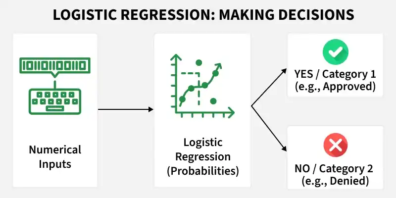
• Logistic Regression uses a linear model combined with the sigmoid function to produce an output between 0 and 1, which can be interpreted as a probability.
• In scikit-learn, you train a model using .fit(X, y).
• You can get the final class predictions with .predict() or, more informatively, the class probabilities with .predict_proba(). The probabilities tell you the model's confidence in each prediction.

Preview of the next lesson:

Now that you can train a classifier, the next logical question is: "How good is it?" In the next lesson, we will explore the essential metrics used to evaluate a classification model, including accuracy, precision, recall, F1-score, and the confusion matrix. This will allow you to measure your model's performance and understand its strengths and weaknesses.