Classifier Evaluation Metrics

1. The Confusion Matrix: Your Evaluation Hub

Before we dive into any specific metrics, we must first understand the confusion matrix. It's a simple table that provides a complete picture of how a model's predictions align with the actual, true labels. All other classification metrics are derived from this matrix, making it the most important concept in this lesson.

A confusion matrix breaks down predictions into four categories. To understand them intuitively, let's watch a short video from StatQuest. It uses a clear example of predicting heart disease.

To solidify this, let's look at another common example: spam detection. Here, "Spam" is our positive class (1) and "Not Spam" is our negative class (0).

Based on this image:

• True Positives (TP) = 5: 5 emails were actually spam, and the model correctly identified them.
• True Negatives (TN) = 7: 7 emails were not spam, and the model correctly identified them.
• False Positives (FP) = 1: 1 email was not spam, but the model incorrectly flagged it as spam.
• False Negatives (FN) = 1: 1 email was spam, but the model failed to catch it.

With these four values, we can now calculate a range of performance metrics.

2. The Core Metrics: Accuracy, Precision, and Recall

While the confusion matrix gives us the raw numbers, we need standardized metrics to quantify and compare model performance. Let's explore the most common ones.

The following video provides a great visual walkthrough of how accuracy, precision, and recall are calculated from the confusion matrix values.

Let's summarize these key metrics:

Accuracy

This is the most straightforward metric. It answers the question: "What proportion of all predictions did the model get right?"

$\text{Accuracy}=\frac{\text{TP}+\text{TN}}{\text{TP}+\text{TN}+\text{FP}+\text{FN}}$

When to use it: When your classes are balanced and you care equally about predicting both positive and negative classes correctly.
When to be cautious: Accuracy can be very misleading on imbalanced datasets. If a disease affects 1% of the population, a model that always predicts "no disease" will be 99% accurate but completely useless for diagnosis.

Precision

Precision focuses on the positive predictions. It answers: "Of all the predictions for the positive class, how many were correct?"

$\text{Precision}=\frac{\text{TP}}{\text{TP}+\text{FP}}$

High precision means your model has a low rate of false positives.

• Example: In spam detection, high precision is vital. You don't want important emails (false positives) being sent to the spam folder. It's better to let a few spam emails through (lower recall) than to lose a critical message.

Recall (or Sensitivity)

Recall also focuses on the positive class, but from a different angle. It answers: "Of all the actual positive cases, how many did the model identify?"

$\text{Recall}=\frac{\text{TP}}{\text{TP}+\text{FN}}$

High recall means your model has a low rate of false negatives.

• Example: In medical diagnosis (e.g., cancer detection), high recall is paramount. You want to identify all actual patients, even if it means some healthy people are wrongly flagged for more tests (lower precision). Missing a true positive case (a false negative) can have severe consequences.

3. The Precision-Recall Trade-off and the F1-Score

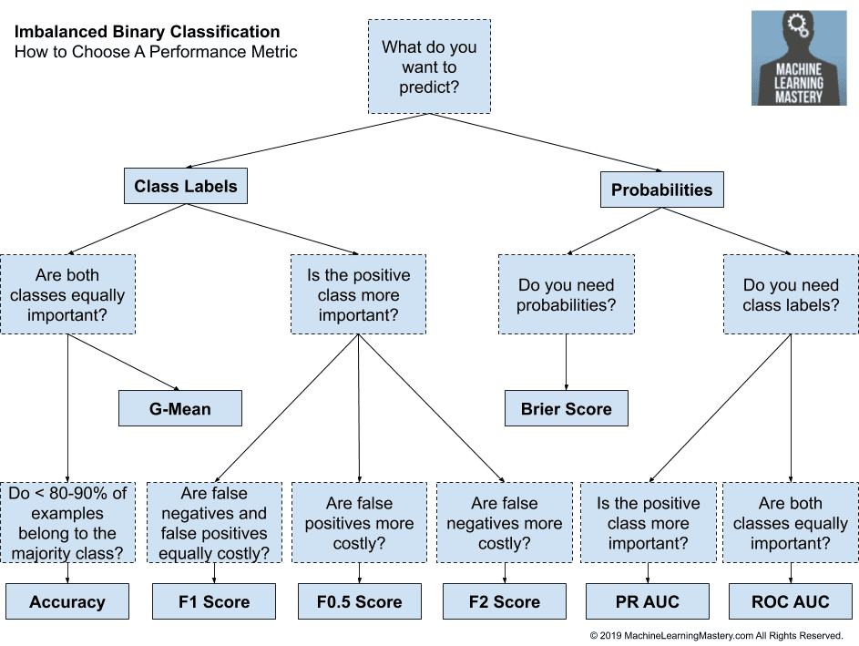
As you can see, there is often a trade-off between precision and recall. Improving one can sometimes hurt the other. Choosing which one to prioritize depends entirely on your project's goal.

The following article provides an excellent discussion of this trade-off using the real-world example of breast cancer detection.

So what do you do when you need a balance between both? That's where the F1-Score comes in.

The F1-Score is the harmonic mean of precision and recall. It provides a single number that balances both metrics. It's particularly useful when you have imbalanced classes and care about minimizing both false positives and false negatives.

$\text{F1-Score}=2\times \frac{\text{Precision}\times \text{Recall}}{\text{Precision}+\text{Recall}}$

The codebasics video you saw earlier also provides a quick explanation of the F1-score.

4. Practical Evaluation with Scikit-learn

Now that you understand the theory, let's turn to the practical side. Scikit-learn's metrics module makes calculating all these metrics incredibly simple. You don't need to manually compute TP, FP, etc.

The most useful function is classification_report, which generates a text summary of all the key metrics for each class.

The following guide provides a clear, code-based walkthrough of how to use scikit-learn's evaluation functions.

To see this in action, the codebasics video concludes with a demonstration of generating a confusion matrix and classification report in Python.

Your Turn: As a practical exercise, I encourage you to go back to the HR analytics exercise from our previous lesson. After you've trained your logistic regression model and made predictions, use confusion_matrix and classification_report to evaluate its performance. Ask yourself: in this context (predicting employee churn), would you prioritize precision or recall?

Conclusion

Great work! You've now built the essential skills to not only build a classification model but also to critically evaluate its performance. This is a crucial step towards building reliable and effective AI systems.

Key Takeaways:

• The Confusion Matrix (TP, TN, FP, FN) is the foundation for evaluating classification models.
• Accuracy is a simple metric but can be misleading, especially with imbalanced data.
• Precision measures the quality of positive predictions (low false positives), while Recall measures the quantity of identified positive cases (low false negatives).
• The choice between prioritizing precision or recall depends on the specific business problem.
• The F1-Score offers a balanced measure when both precision and recall are important.
• Scikit-learn's classification_report provides a convenient and comprehensive summary of these metrics.

Preview of the next lesson:

Now that you know how to build and evaluate a classifier, we will expand your modeling toolkit. In the next lesson, we will explore a completely different type of classification algorithm: K-Nearest Neighbors (KNN). It's an intuitive, instance-based model, and you'll be able to use the metrics you learned today to compare its performance against the logistic regression model.