KNN Classifier: Training and Mechanism

1. The Core Mechanism of K-Nearest Neighbors

The central idea behind KNN is simple and can be summed up by the old saying: "You are the company you keep." To classify a new, unknown data point, KNN looks at the other data points in its neighborhood and makes a decision based on the majority.

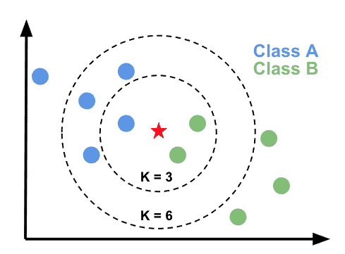
This simple idea has a few key components that define how the algorithm works.

A "Lazy" Learner

Unlike logistic regression, which learns a set of weights (coefficients) during the fit process, KNN doesn't really "learn" a model in the same way. Instead, it simply stores, or memorizes, the entire training dataset. This is why it's called a lazy learning or instance-based algorithm. The actual computation—finding the nearest neighbors—is deferred until a prediction is requested.

To get a deeper understanding of KNN's mechanics, including the crucial role of the 'K' parameter, watch the following video.

As the video explained, the two most important elements to configure for a KNN model are:

1. The Number of Neighbors (K): This is a hyperparameter you must choose.

   • A small K (e.g., K=1) makes the model highly sensitive to noise and outliers, potentially leading to overfitting.
   • A large K makes the decision boundary smoother but can include points from other classes, leading to underfitting.
   • A common practice is to start with an odd number for K (like 3, 5, or 7) to avoid ties in binary classification. We'll explore how to find the optimal K in a later module.

2. The Distance Metric: This defines what "nearest" means. The most common metric is Euclidean distance—the straight-line distance between two points. For two points ${\mathbf{x}}_q$ and ${\mathbf{x}}_i$ in an n-dimensional space, the formula is:
   $d({\mathbf{x}}_q,{\mathbf{x}}_i)=\sqrt{{\sum }_{j=1}^n(x_{q,j}-x_{i,j}{)}^2}$
   This is essentially the Pythagorean theorem generalized to more than two dimensions. While other metrics exist (like Manhattan or Cosine distance), Euclidean is the default in scikit-learn and a great starting point.

2. The Critical Importance of Feature Scaling

Because KNN relies entirely on distance, it's highly sensitive to the scale of your features.

Imagine you have a dataset with two features: age (ranging from 20-70) and salary (ranging from 50,000-200,000). When calculating the distance, the salary feature, with its much larger range, will completely dominate the calculation. The differences in age will become almost irrelevant.

To prevent this, you must scale your features before training a KNN model. This ensures that all features contribute equally to the distance calculation. A common technique is Standardization, which transforms each feature to have a mean of 0 and a standard deviation of 1.

The following article demonstrates this step in a practical workflow.

3. Practical Implementation with Scikit-learn

Now let's put it all together and build a KNN classifier. Your background in Python and familiarity with scikit-learn's interface will make this very straightforward. We'll follow a video tutorial that uses the Iris dataset, a classic dataset for classification tasks.

First, let's focus on the model training process.

The core steps to train a KNN model are:

1. Import necessary classes:

   from sklearn.model_selection import train_test_split
   from sklearn.preprocessing import StandardScaler
   from sklearn.neighbors import KNeighborsClassifier
   

2. Split your data:

   X_train, X_test, y_train, y_test = train_test_split(X, y, test_size=0.3, random_state=42)
   

3. Scale your features:

   scaler = StandardScaler()
   X_train_scaled = scaler.fit_transform(X_train)
   X_test_scaled = scaler.transform(X_test) # Use the same scaler fitted on the training data
   

4. Initialize and train the model:

   knn = KNeighborsClassifier(n_neighbors=5) # Initialize with K=5
   knn.fit(X_train_scaled, y_train)
   

4. Evaluating the KNN Model

Once the model is trained, we can evaluate its performance using the metrics you learned in the previous lesson. This workflow—train, predict, evaluate—is central to applied machine learning.

Let's see how this is done in the video.

As you saw, evaluating the model involves:

1. Making predictions on the scaled test set.
2. Using scikit-learn's metrics functions with the true labels (y_test) and the predicted labels.

from sklearn.metrics import confusion_matrix, classification_report, accuracy_score




# Make predictions
y_pred = knn.predict(X_test_scaled)




# Calculate accuracy
print(f"Accuracy: {accuracy_score(y_test, y_pred):.2f}")




# Display the confusion matrix
print("\nConfusion Matrix:")
print(confusion_matrix(y_test, y_pred))




# Display the classification report
print("\nClassification Report:")
print(classification_report(y_test, y_pred))

This process allows you to objectively assess your model and compare it to others, like the logistic regression model you built earlier.

Your Turn: Practice Exercise

Learning machine learning is like learning to swim; you have to get in the water. The codebasics video concludes with an excellent exercise that will help you solidify your understanding.

Advanced Tip: The exercise asks you to find the optimal value of K. You can do this by manually trying a few values, or you can use a more systematic approach like cross-validation. The GeeksforGeeks article (LINK), in its Section 4, shows how to write a loop with cross_val_score to plot accuracy for different K values. This is a powerful technique you will learn formally in a future module.

Conclusion

Fantastic work! You've successfully added another powerful classifier to your skillset. You not only know how KNN works under the hood but can also implement and evaluate it effectively using standard industry tools.

Key Takeaways:

• KNN is an intuitive instance-based or "lazy" learning algorithm.
• It classifies new data by taking a majority vote from its 'K' nearest neighbors.
• The core mechanism depends on the number of neighbors (K) and the distance metric (usually Euclidean).
• Feature scaling is mandatory for KNN to ensure all features contribute fairly to the distance calculation.
• The implementation workflow in scikit-learn involves StandardScaler and KNeighborsClassifier.

Preview of the next lesson:
So far, we've seen a model based on a linear equation (Logistic Regression) and a model based on distance (KNN). In the next lesson, we will explore a third type: Decision Trees. This algorithm makes predictions by learning a hierarchy of "if/else" rules from the data, resulting in a model that is highly interpretable and easy to visualize.