Decision Tree Classification and Visualization

1. The Logic of a Decision Tree: A "White Box" Model

Unlike models that can feel like a "black box" (where the decision-making process is hard to inspect), decision trees are often called "white box" models. They provide a clear, visual flowchart of the logic they used to arrive at a prediction.

The core idea is to recursively split the data into smaller, more homogeneous groups based on the features. At each step, the algorithm asks a question about a feature to create the "purest" possible split. But what does "pure" mean?

This is determined by a metric that measures the level of impurity or disorder in a group of data points. The goal is to find splits that decrease this impurity as much as possible. Two common metrics are:

• Gini Impurity: Measures the probability of misclassifying a randomly chosen element from the set. A Gini score of 0 means the set is perfectly pure (all elements belong to one class). A score of 0.5 (in a binary classification problem) means the set is maximally impure (a 50/50 split of classes).
• Entropy: Originating from information theory, entropy also measures the amount of disorder. An entropy of 0 indicates a perfectly pure set.

Scikit-learn's DecisionTreeClassifier uses the Gini index by default. To understand these concepts more formally, please read the following section from a DataCamp tutorial.

In essence, at every node, the tree searches through every feature and every possible split point for that feature. It calculates the Gini impurity for each potential split and chooses the one that results in the lowest weighted average impurity for the resulting child nodes.

2. Training a Decision Tree with Scikit-learn

Now that you have the conceptual foundation, let's move to the practical implementation. Given your experience with scikit-learn's API, you'll find this process familiar.

The steps are standard: import the classifier, create an instance, and use the .fit() method.

# 1. Import necessary libraries
from sklearn.datasets import load_breast_cancer
from sklearn.model_selection import train_test_split
from sklearn.tree import DecisionTreeClassifier
from sklearn.metrics import accuracy_score




# 2. Load and split the data
data = load_breast_cancer()
X = data.data
y = data.target
feature_names = data.feature_names
class_names = data.target_names

X_train, X_test, y_train, y_test = train_test_split(X, y, test_size=0.3, random_state=42)




# 3. Initialize and train the classifier
# We'll start with default parameters
clf = DecisionTreeClassifier(random_state=42)
clf.fit(X_train, y_train)




# 4. Make predictions and evaluate
y_pred = clf.predict(X_test)
accuracy = accuracy_score(y_test, y_pred)
print(f"Accuracy: {accuracy:.4f}")

Running this code will train a decision tree and report its accuracy. However, this doesn't yet help us understand the logic it learned. For that, we need visualization.

3. Visualizing and Interpreting the Tree

This is where the power of decision trees truly shines. We can plot the entire tree structure to see exactly how it makes decisions. Scikit-learn provides a function called plot_tree for this purpose.

The video below provides an excellent walkthrough of how to generate this plot and, more importantly, how to interpret what each part of it means.

Let's break down a node using an example visualization to solidify your understanding.

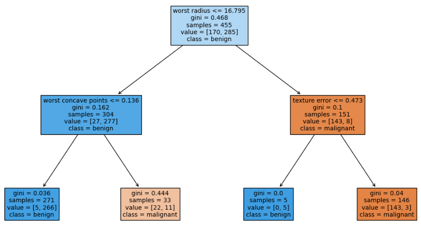
Let's analyze the root node (the very top one):

1. worst radius <= 16.795: This is the decision rule. For any data point, if its 'worst radius' feature is less than or equal to 16.795, it goes down the left branch (True). Otherwise, it goes down the right branch (False).
2. gini = 0.463: This is the Gini impurity of the node. Since this is the root node containing all 398 training samples, it's not pure.
3. samples = 398: This tells us how many training samples are in this node.
4. value = [149, 249]: This shows the distribution of classes among the samples in this node. Here, there are 149 samples of the first class ('malignant') and 249 of the second class ('benign').
5. class = benign: This is the prediction the model would make if it stopped at this node. It's simply the majority class in the value array.

By following the path from the root node down to a leaf node (a node with no children), you can trace the exact sequence of rules that leads to a final classification. This transparency is a key advantage of decision trees.

4. Controlling Complexity to Avoid Overfitting

If you were to plot the tree we trained in the code snippet from section 2, you would see a very large, complex tree. By default, a decision tree will keep splitting the data until every leaf node is perfectly pure (or contains only one sample). While this results in 100% accuracy on the training data, it almost always leads to overfitting. The model learns the noise and quirks of the training set too well and fails to generalize to new, unseen data.

To combat this, we can control the tree's complexity, a process called pruning. The simplest way is pre-pruning, where we stop the tree from growing too deep by setting constraints.

One of the most important parameters for this is max_depth. Let's see how setting this hyperparameter can give us a more manageable and often better-performing model.

By limiting the depth, we force the model to only learn the most important patterns in the data, making it more robust. Other useful pre-pruning parameters include:

• min_samples_split: The minimum number of samples a node must have before it can be split.
• min_samples_leaf: The minimum number of samples a leaf node must have.

Conclusion

Great job today! You have now learned how to train, visualize, and interpret a decision tree classifier. This is a significant step in building your practical machine learning skills, as interpretability is highly valued in many real-world applications.

Key Takeaways:

• Decision trees are "white box" models that classify data using a series of if-then-else rules.
• The logic for splitting is based on minimizing impurity, typically measured by the Gini Index or Entropy.
• You can train a DecisionTreeClassifier in scikit-learn using the familiar .fit() method.
• The sklearn.tree.plot_tree function is essential for visualizing the tree's logic, allowing you to inspect every decision rule.
• Uncontrolled trees are prone to overfitting. You can control their complexity using pre-pruning techniques, such as setting the max_depth hyperparameter.

Preview of the next lesson:
All the datasets we've used so far have had a relatively balanced number of samples for each class. But what happens when one class is much rarer than another (e.g., fraud detection, where fraudulent transactions are a tiny fraction of the total)? In our next lesson, we will tackle this problem by learning about handling class imbalance, starting with a technique called stratified splitting.