Model Selection and Justification

1. Beyond a Single Score: A Framework for Model Selection

In our previous step, we ranked models using their cross-validated MAE. This is a great start, but a single number can hide important details. For instance:

• What if the model with the best average score is also the most unstable, with performance varying wildly depending on the data it sees?
• What if the top two models have nearly identical scores, but one is much simpler and faster to train?
• What if we need to explain why a prediction was made, and our top model is a complete "black box"?

To make a final choice, we need to evaluate our candidates across several dimensions.

Here's a structured approach to think about your final selection:

1. Broader Performance Metrics: Go beyond MAE. Let's include metrics like Root Mean Squared Error (RMSE), which penalizes large errors more heavily, and the R-squared (R²) score, which tells us the proportion of variance in the salary that our model can explain.
2. Performance Stability: A model's average score is important, but so is its variance. The standard deviation of scores from our cross-validation folds gives us a measure of this stability. A lower standard deviation indicates a more reliable model.
3. Model Complexity & Training Time: Simpler is often better. If a simple model performs almost as well as a complex one, it might be preferred because it's faster, easier to deploy, and less prone to overfitting. We can use training time as a proxy for complexity.
4. Interpretability: Can you explain a model's predictions? Models like Ridge regression are highly interpretable. Ensemble models like RandomForestRegressor are less so, but they offer tools like feature importance plots, which tell us which features most influenced their predictions.

The following article provides a great overview of this multi-faceted evaluation process.

2. Deepening the Evaluation with Code

Let's put this framework into practice. We'll now augment the test harness from our previous lesson to collect multiple metrics and visualize more diagnostics for our top-performing models.

Expanding the Test Harness

We can use sklearn.model_selection.cross_validate (instead of cross_val_score) to compute multiple metrics in a single run. This is much more efficient.

Let's compare our top three contenders from last time: Ridge, RandomForestRegressor, and GradientBoostingRegressor.

# Assuming X and y are your prepared feature matrix and target vector




# 1. Import libraries
from sklearn.model_selection import cross_validate
from sklearn.linear_model import Ridge
from sklearn.ensemble import RandomForestRegressor, GradientBoostingRegressor
import numpy as np
import pandas as pd




# 2. Define models to compare
models = {
    "Ridge": Ridge(),
    "RandomForest": RandomForestRegressor(n_estimators=100, random_state=42),
    "GradientBoosting": GradientBoostingRegressor(random_state=42)
}




# 3. Define metrics to calculate
scoring_metrics = ['neg_mean_absolute_error', 'neg_root_mean_squared_error', 'r2']




# 4. Evaluate models
results = {}
for name, model in models.items():



    # Use cross_validate to get multiple scores and fit_time
    cv_results = cross_validate(model, X, y, cv=10, scoring=scoring_metrics, return_train_score=False)
    results[name] = cv_results




# 5. Summarize and display results in a table
summary_data = []
for name, res in results.items():
    mae = -res['test_neg_mean_absolute_error'].mean()
    mae_std = res['test_neg_mean_absolute_error'].std()
    rmse = -res['test_neg_root_mean_squared_error'].mean()
    r2 = res['test_r2'].mean()
    fit_time = res['fit_time'].mean()
    
    summary_data.append({
        "Model": name,
        "MAE": f"${mae:,.2f} ± ${mae_std:,.2f}",
        "RMSE": f"${rmse:,.2f}",
        "R-squared": f"{r2:.3f}",
        "Avg Fit Time (s)": f"{fit_time:.2f}"
    })

summary_df = pd.DataFrame(summary_data)
print(summary_df)

Running this code will produce a clear, comprehensive table comparing your models across several key dimensions, making your decision process much more structured.

3. Visual Diagnostics: Learning Curves and Feature Importance

Numbers are essential, but visualizations often provide deeper insights.

Learning Curves

As you'll recall from Module 4, learning curves plot model performance against the amount of training data. They are the best tool for diagnosing whether a model is suffering from high bias (underfitting) or high variance (overfitting).

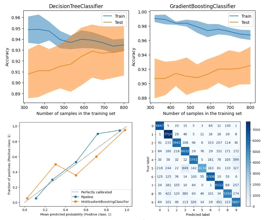
You can generate these curves for your top two models (e.g., RandomForest and GradientBoosting) to see if one generalizes better than the other. You can reuse the code for plotting learning curves from our lesson in Module 4, [5] Plot and interpret learning curves to diagnose bias and variance issues.

Feature Importance

For tree-based ensemble models, we can easily check which features they found most predictive. This is a great sanity check and adds a layer of interpretability. If the model highlights features that you identified as important during EDA, it increases your confidence in the model.

Here’s how you can train a RandomForestRegressor and plot its feature importances:

import matplotlib.pyplot as plt




# Train the final chosen model on the full training data
# (Let's assume we chose RandomForest for this example)
final_model = RandomForestRegressor(n_estimators=100, random_state=42)
final_model.fit(X, y)




# Get feature importances
importances = final_model.feature_importances_
feature_names = X.columns # Assuming X is a pandas DataFrame




# Create a pandas series for easy plotting
feat_importances = pd.Series(importances, index=feature_names)




# Plot
plt.figure(figsize=(10, 8))
feat_importances.nlargest(15).plot(kind='barh')
plt.title("Top 15 Most Important Features")
plt.xlabel("Relative Importance")
plt.show()

4. Your Turn: Select and Justify Your Final Model

Now it's time to bring all these pieces together.

Your Task:

1. Generate the Comparison Table: Run the provided code snippet to create a summary table of performance metrics (MAE, RMSE, R²) and fit times for the Ridge, RandomForest, and GradientBoosting models.
2. Plot Learning Curves: Generate and compare the learning curves for your top two models (likely RandomForest and GradientBoosting). Does one show signs of overfitting more than the other?
3. Plot Feature Importances: For your top-performing ensemble model, generate the feature importance plot. Do the results make sense based on your domain knowledge and EDA?
4. Write Your Justification: Based on all the evidence you've gathered (the table, learning curves, and feature importances), select one final model. Write a short paragraph in your notebook justifying your choice.

Your justification should be a narrative. Don't just state the winner. Explain the trade-offs you considered. For example:

"While the Gradient Boosting model achieved a slightly lower MAE ($X) compared to the Random Forest ($Y), I have selected the Random Forest as the final model. The learning curves showed that the Random Forest generalized slightly better, with a smaller gap between training and validation scores. Furthermore, its performance was more stable across cross-validation folds (lower standard deviation in MAE) and it trained significantly faster. Given the marginal performance difference, the Random Forest's superior stability and efficiency make it the more practical choice for this project. Its feature importances also confirmed that 'Years of Experience' and 'Job Title' were the most predictive variables, aligning with our initial hypotheses."

Conclusion

Excellent work! You've gone from a simple leaderboard to a comprehensive, evidence-based decision. This process of systematic evaluation and justification is a hallmark of a professional data scientist. It ensures your model choice is not arbitrary but is instead robust, well-reasoned, and aligned with project goals.

Key Takeaways:

• Comprehensive evaluation is key: Don't rely on a single metric. Assess models based on performance, stability, complexity, and interpretability.
• Use summary tables for clarity: A well-structured table makes it easy to compare models across multiple criteria.
• Visual diagnostics are powerful: Learning curves help diagnose bias and variance, while feature importance plots provide crucial interpretability.
• Justify your choice: A written justification demonstrates your reasoning and communicates the trade-offs you considered when selecting the final model.

Preview of the next lesson:
Now that you have selected and justified your final model, the next step is to understand its behavior at a deeper level. In our next lesson, we will interpret the predictions of the final model using a technique like SHAP, moving from "what did the model predict?" to "why did it make that prediction?".