Model Training and Evaluation

1. The Starting Point: Why We Need a Baseline

Before we start building complex models, we need a reference point. How do we know if a model is actually "good"? A model with a Mean Absolute Error (MAE) of $50,000 might sound poor, but if a naive guess is off by $100,000, then our model is providing significant value. This is the role of a baseline.

A baseline is a simple, often non-ML model that provides a "common sense" prediction. For a regression task like ours, a common baseline is to simply predict the average salary for every single person. If our sophisticated machine learning models can't perform better than this simple average, it's a strong signal that they aren't learning meaningful patterns from the data.

This short video explains the strategic importance of baselines in any machine learning project.

Implementing a Baseline in Scikit-Learn

For regression tasks, Scikit-learn provides a handy tool called DummyRegressor that does exactly what we need. We can configure it to always predict the mean of the target variable from the training set.

Let's see how to implement and evaluate it alongside a slightly more complex model, like a Decision Tree.

This establishes our first two models: the DummyRegressor as our baseline and a DecisionTreeRegressor as our first real candidate.

2. Choosing Your Next Models

With a baseline set, how do we select other, more complex models to test? The world of machine learning algorithms is vast, but we can make informed choices. The Scikit-learn algorithm cheat sheet is an excellent guide for this.

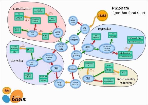
Following the path for our regression problem:

• Start -> >50 Samples -> Yes.
• Predicting a category? -> No.
• Predicting a quantity? -> Yes.
• Not all features are important? -> This leads to algorithms with built-in feature selection like Lasso and ElasticNet.
• If that's not the case, the map suggests RidgeRegression and SVR (with a linear kernel).
• If those don't work, it points towards ensemble methods like RandomForestRegressor and GradientBoostingRegressor.

Based on this, good candidates to try in addition to our Decision Tree would be:

• Linear Models: Ridge (a regularized version of linear regression).
• Ensemble Models: RandomForestRegressor and GradientBoostingRegressor. These models are often very powerful on structured, tabular data like ours.

3. Building a Fair Comparison: The Test Harness

To evaluate these different models, we can't just train each one on all the data and see which has the lowest training error. That would lead to overfitting. Instead, we must create a test harness—a standardized process that evaluates each model consistently. The key is using cross-validation, which you learned about in Module 4.

The following article provides a complete, practical template for creating such a test harness in Python.

The example in the article is for a classification problem (predicting diabetes), but the structure is directly applicable to our regression problem. We just need to swap out the models and the scoring metric.

4. Your Turn: Train and Evaluate Your Models

Now it's time to apply these concepts to our salary prediction project. You will adapt the test harness from the article to compare our chosen models.

Here is a Python code structure to guide you. Assume you have your feature matrix X and target vector y ready from the previous lesson.

# 1. Import libraries
import pandas as pd
import matplotlib.pyplot as plt
from sklearn.model_selection import KFold, cross_val_score




# Import the models
from sklearn.dummy import DummyRegressor
from sklearn.tree import DecisionTreeRegressor
from sklearn.linear_model import Ridge
from sklearn.ensemble import RandomForestRegressor, GradientBoostingRegressor




# 2. Prepare models
models = []
models.append(('Baseline', DummyRegressor()))
models.append(('CART', DecisionTreeRegressor()))
models.append(('Ridge', Ridge()))
models.append(('RF', RandomForestRegressor(n_estimators=100))) # n_estimators is a common hyperparameter to set
models.append(('GBM', GradientBoostingRegressor()))




# 3. Evaluate each model in turn
results = []
names = []
scoring = 'neg_mean_absolute_error' # Use a regression metric. Lower is better, but scikit-learn maximizes, so we use the negative.

for name, model in models:
    kfold = KFold(n_splits=10, random_state=42, shuffle=True) # Use a fixed random_state for reproducibility
    cv_results = cross_val_score(model, X, y, cv=kfold, scoring=scoring)
    results.append(cv_results)
    names.append(name)



    # We print the negative of the mean because the metric is negative MAE
    print(f"{name}: {-cv_results.mean():.2f} ({-cv_results.std():.2f})")




# 4. Compare algorithms using a boxplot
fig = plt.figure()
fig.suptitle('Algorithm Comparison')
ax = fig.add_subplot(111)



# We plot the absolute values of the scores to see the actual MAE
plt.boxplot([-r for r in results])
ax.set_xticklabels(names)
plt.ylabel('Mean Absolute Error (MAE)')
plt.show()

Your Task:
Integrate this code into your project notebook. Run the evaluation and analyze the output.

• Which model performs best on average (lowest mean MAE)?
• Which model is the most stable (smallest standard deviation and tightest boxplot)?
• How much better is your best model compared to the Baseline? This quantifies the value of your modeling efforts.

Conclusion

Congratulations! You've successfully trained and evaluated your first set of machine learning models for this project. You have moved from raw data to concrete performance metrics, a major milestone in any data science workflow.

Key Takeaways:

• Always start with a baseline: Use a simple model like DummyRegressor to establish a performance floor. Any useful model must beat this.
• Systematic model selection: Use tools like the Scikit-learn flowchart to choose a variety of candidate models (e.g., linear, tree-based, ensemble).
• Fair evaluation is critical: A test harness using cross-validation ensures that all models are compared under the same conditions, giving you a robust estimate of their performance on unseen data.
• Visualize your results: Boxplots are an excellent tool for comparing both the average performance (median line) and the variance (box size) of your models.

Preview of the next lesson:
You now have a leaderboard of models. But which one should you choose? The model with the absolute best score isn't always the right answer. In our next lesson, we will learn how to select and justify the final model based on a comprehensive evaluation, considering factors beyond just a single performance metric.