Hello! Welcome back to our end-to-end data science project.
In our last lesson, we took the crucial first step of framing our project: translating the business need for salary transparency into a defined machine learning problem—a regression task to predict data scientist salaries.
Today, we transition from planning to execution. Our learning outcome is to execute a full project workflow: EDA, preprocessing, and feature engineering on a new dataset. This is where you'll bring together the skills you've built in earlier modules and apply them in a connected, practical sequence. You'll see how a raw dataset is methodically explored, cleaned, and enriched to prepare it for modeling.
Let's dive into the data and begin the hands-on work.
1. The Project Workflow: A Bird's-Eye View
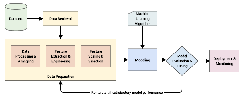
Before we start coding, it's helpful to visualize where today's tasks fit into the larger machine learning lifecycle. The initial phase of any project is about preparing the data, which is exactly our focus.
This preparation phase is not a single step but an iterative process of its own, often called Exploratory Data Analysis (EDA).
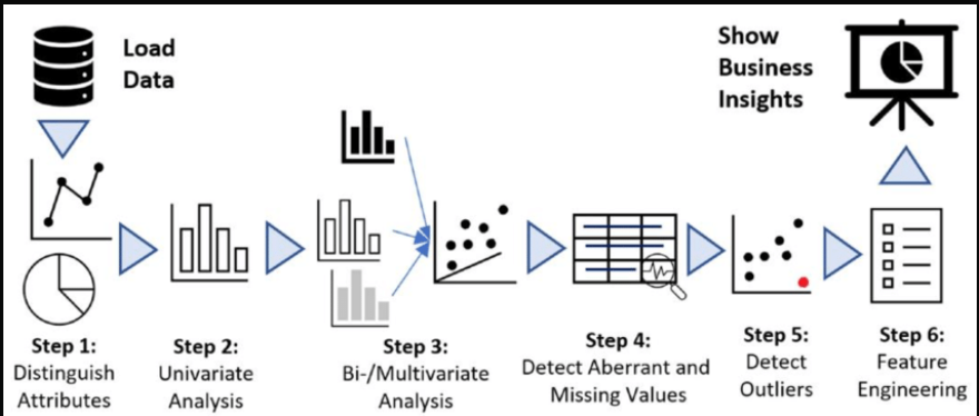
We will follow this workflow using two excellent, practical video demonstrations from experienced data scientists.
2. Step 1: Data Understanding and Preparation
The first phase involves getting a feel for the dataset. This includes loading the data, performing initial inspections, and cleaning it up. We'll watch a video that provides a clear, step-by-step walkthrough of this process.
Exploratory Data Analysis with Pandas Python
In this video, 'Exploratory Data Analysis with Pandas Python,' Kaggle Grandmaster Rob Mulla demonstrates his typical workflow when encountering a new dataset. We will focus on the initial data understanding and preparation stages.
Please watch the following segments carefully: Data Understanding (03:29 - 06:38): Pay attention to the first commands he runs: .shape, .head(), .columns, .dtypes, and .describe(). These are your essential first-look tools. Data Preparation - Subsetting (06:38 - 11:23): Observe how he selects a relevant subset of columns for the analysis. In a real project, you rarely use every single column. Data Preparation - Cleaning (11:23 - 20:57): This is a critical section. Focus on the techniques for renaming columns for consistency (.rename()), changing data types (pd.to_datetime), finding missing values (.isnull().sum()), and handling duplicate rows (.duplicated(), .drop_duplicates()).
These initial steps are foundational. A clean, well-understood dataset prevents countless issues down the line. Notice how the process is a cycle: you inspect the data (.head(), .dtypes), find an issue (e.g., a messy column name or wrong data type), and then clean it (.rename(), pd.to_datetime).
3. Step 2: Feature Engineering
With a cleaned dataset, we can now move to one of the most creative and impactful stages: feature engineering. This is the process of using your domain knowledge to create new features from existing ones, providing more meaningful signals to your model.
The following article provides a concise overview of what feature engineering is and why it's so important.
Feature Engineering in Machine Learning: A Practical Guide
This article, 'Feature Engineering in Machine Learning,' gives a great introduction to the topic and illustrates its power.
Please read two short sections: 'What is Feature Engineering in Machine Learning?': This will give you a clear definition and a real-world example of its impact. 'Creating new features': This section provides a simple, intuitive example of deriving a new feature (area) from existing ones (length, breadth).
Now, let's see this in action. We'll watch a video from data scientist Ken Jee, who happens to be working on the exact salary prediction problem we defined in our last lesson. His feature engineering steps are directly relevant to our project.
Data Science Project from Scratch - Part 4 (Exploratory Data Analysis)
In this video, 'Data Science Project from Scratch - Part 4 (Exploratory Data Analysis),' Ken Jee demonstrates several practical feature engineering techniques on a salary dataset.
Watch the section on Feature Engineering (03:09 - 12:27). Notice how he transforms raw data into useful features: Simplifying job titles (e.g., 'sr data scientist' -> 'data scientist'). Extracting seniority (e.g., 'sr', 'jr') into a new column. Calculating the length of the job description. Counting the number of competitors from a string. These are perfect examples of creating new, structured information from unstructured or complex data.
Think about it: How could you apply these ideas to our project? If you had a Year Founded column for a company, what new feature could you create that might be more predictive of salary? (Hint: Company age!).
4. Step 3: Univariate and Multivariate Analysis
After cleaning the data and engineering new features, we return to analysis, but this time with visualizations to uncover deeper patterns. We'll analyze single variables (univariate) and relationships between variables (bivariate/multivariate).
For a comprehensive textual guide on the different types of analysis and the plots used for each, the following article is an excellent resource.
Exploratory Data Analysis (EDA) Using Python - Analytics Vidhya
The article 'Exploratory Data Analysis (EDA) Using Python' from Analytics Vidhya provides a structured overview of the analysis phase.
Skim through the following sections to get a structured overview of the analysis types. You don't need to read the code in detail, but focus on the concepts: Step 7: EDA Exploratory Data Analysis: A quick recap of what EDA is. Step 9: EDA Univariate Analysis: Understand the goal of analyzing one variable at a time (e.g., using histograms for numerical data, count plots for categorical). Step 12: EDA Bivariate Analysis: Understand how to explore relationships between two variables (e.g., using scatter plots). Step 13: EDA Multivariate Analysis: See how heatmaps are used to visualize correlations between many variables at once.
Now, let's return to Rob Mulla's video to see these visualization techniques applied in a fluid, practical workflow.
Exploratory Data Analysis with Pandas Python
We'll continue with Rob Mulla's video to see how he uses visualizations to explore the cleaned data.
Watch the final analysis segments of the video: Univariate Analysis (20:57 - 27:44): Focus on how he uses .value_counts() and plots (histograms, KDE plots) to understand the distribution of individual features like 'Year Introduced' and 'Speed'. Feature Relationships (27:44 - 35:26): This is a great demonstration of bivariate and multivariate analysis. Observe his use of: Scatter plots to compare two numerical features (e.g., Speed vs. Height). Pair plots (seaborn.pairplot) to quickly visualize relationships across multiple features. Correlation Heatmaps (seaborn.heatmap) to get a quantitative summary of linear relationships.
These visualizations are not just for making pretty charts. They help you build intuition about your data, formulate hypotheses (e.g., "It seems like faster roller coasters are also taller"), and spot potential issues like outliers or multicollinearity that you'll need to address before modeling.
Conclusion
In this lesson, you've walked through the essential first phase of a hands-on data science project. You've seen how a raw dataset is systematically analyzed, cleaned, and enriched to make it ready for a machine learning model. This workflow is the bedrock of any successful modeling endeavor.
Key Takeaways:
- The initial project phase is an iterative cycle of data understanding, cleaning, feature engineering, and visualization.
- Data understanding starts with basic pandas commands like
.shape,.head(),.info(), and.describe(). - Data cleaning involves handling missing values, correcting data types, dealing with duplicates, and standardizing column names.
- Feature engineering is the art of creating new, predictive features from existing data to improve model performance.
- Visual analysis (univariate, bivariate, multivariate) is crucial for identifying patterns, spotting outliers, and understanding relationships between variables using tools like histograms, scatter plots, and heatmaps.
Preview of the next lesson:
With our data now explored and prepared, we are ready for the next exciting step. In the next lesson, we will train and evaluate a baseline model and at least two more complex candidate models. This is where we'll see if our hard work in data preparation pays off