Interpreting Model Predictions with SHAP

1. Beyond "What" to "Why": Introducing SHAP

Your final model, likely a RandomForestRegressor or GradientBoostingRegressor, is powerful but can feel like a "black box." It gives you a prediction, but doesn't immediately tell you how it arrived at that number. What if you need to explain to a manager why one employee's predicted salary is $20,000 higher than another's?

This is where SHAP (SHapley Additive exPlanations) comes in. SHAP is a state-of-the-art method rooted in cooperative game theory that explains any machine learning model's output.

The core idea is to treat features as "players" in a game, where the "payout" is the model's prediction. SHAP calculates the unique contribution of each player (feature) to that payout.

This video from DeepFindr provides a great introduction to the game theory intuition behind SHAP.

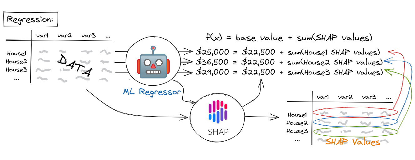
The key takeaway is that for any single prediction, SHAP can decompose it like this:

Final Prediction = Average Prediction (Base Value) + Sum of Contributions from each Feature

Each feature's contribution is its SHAP value. A positive SHAP value means that feature pushed the prediction higher than the average, while a negative SHAP value means it pushed the prediction lower.

2. Hands-On: Calculating SHAP Values for Your Model

Let's apply this to the salary prediction model you finalized in the last lesson. Your hands-on work has shown your comfort with Python, so we'll dive right into the implementation.

First, you need to install the shap library:

pip install shap

Now, assuming you have your finalized model (final_model) and your test data (X_test), we can calculate the SHAP values.

import shap
import pandas as pd




# Let's assume 'final_model' is your trained RandomForest or GradientBoosting model
# and 'X_test' is your test set of features.




# 1. Create an explainer object
# We use TreeExplainer because it's highly optimized for tree-based models
# like Random Forest and Gradient Boosting.
explainer = shap.TreeExplainer(final_model)




# 2. Calculate SHAP values for your test data
# This can take a moment for larger datasets.
shap_values = explainer.shap_values(X_test)




# The result 'shap_values' is a numpy array where each row corresponds
# to a sample in X_test, and each column corresponds to a feature.
# Let's wrap it in a DataFrame for easier inspection.
shap_df = pd.DataFrame(shap_values, columns=X_test.columns)

print("SHAP values calculated for all test instances.")
print("Shape of SHAP values:", shap_df.shape)
print("Shape of X_test:", X_test.shape)

Run this code in your project notebook. You now have the specific contribution of every feature for every prediction in your test set.

3. Local Explanations: Explaining a Single Prediction

This is where the power of SHAP truly shines. Let's pick one specific data scientist from your test set and explain their salary prediction.

The Waterfall Plot

The waterfall plot is one of the most intuitive ways to visualize a single explanation.

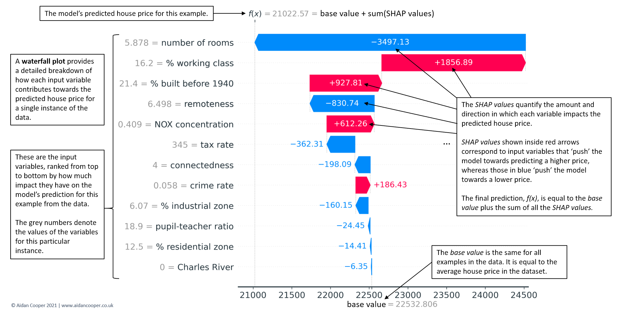
Let's generate one for the first person in your test set. The explainer.expected_value gives us the base value (the average predicted salary).

# Initialize javascript plotting in your notebook
shap.initjs()




# Explain the prediction for the first instance in the test set
shap.plots.waterfall(explainer.expected_value, shap_values[0], X_test.iloc[0])

Your Task (Part 1):

1. Run the code above to generate the waterfall plot for the first instance.
2. Interpret the plot:
   • What is the base (average) predicted salary?
   • What is the final predicted salary for this specific person?
   • Which feature had the biggest positive impact (pushed the salary up the most)?
   • Which feature had the biggest negative impact (pushed it down the most)?
3. Now, pick another instance from your test set (e.g., shap_values[10], X_test.iloc[10]) and generate a new waterfall plot. How does the explanation differ?

This exercise moves you from theory to practice, allowing you to see how different feature values lead to different outcomes.

4. Global Explanations: Summarizing Model Behavior

While explaining individual predictions is powerful, we also want to understand the model's behavior across the entire dataset. SHAP provides visualizations for this that are far more insightful than the standard feature importance plot you used previously.

This next video provides an excellent, code-first walkthrough of the most important SHAP plots. We'll focus on the summary plot (beeswarm) and dependence plot.

The Beeswarm (Summary) Plot

The beeswarm plot is arguably the most useful summary SHAP provides. It shows not only which features are most important but also how their value affects the prediction.

# Generate the summary plot
shap.summary_plot(shap_values, X_test)

How to read this plot:

• Feature Importance: Features are ranked by importance on the y-axis.
• Impact: The x-axis is the SHAP value. Points to the right of zero show a positive impact on the prediction; points to the left show a negative impact.
• Original Value: The color represents the feature's value for that instance—high values are red, low values are blue.
• Distribution: Each dot is a person in your test set. The density of dots shows the distribution of effects.

For example, you might see a cluster of red dots for "Years of Experience" on the far right of the plot. This would tell you that high years of experience consistently and strongly push salary predictions higher.

The Dependence Plot

To zoom in on the effect of a single feature, we can use a dependence plot. It shows how a feature's value (x-axis) relates to its SHAP value (y-axis). We can even color the points by a second feature to uncover interaction effects.

# Create a dependence plot for the most important feature
# Replace 'Years of Experience' with the top feature from your summary plot
shap.dependence_plot('Years of Experience', shap_values, X_test)




# To check for interactions, color it by another feature
# Replace 'Job Title Encoded' with another relevant feature
shap.dependence_plot('Years of Experience', shap_values, X_test, interaction_index='Job Title Encoded')

Your Task (Part 2):

1. Generate the summary_plot for your model.
2. Write down two key insights you can draw from it. For example, "Low values of feature X have a strong negative impact on salary" or "Feature Y has a wide range of impacts, suggesting it interacts with other features."
3. Generate a dependence_plot for your most important feature. Does it show a linear relationship, or something more complex?

Conclusion

Congratulations! You've successfully peered inside the "black box" of your model. This is a massive step in your journey from being someone who can build models to someone who can understand and explain them. This ability is what separates junior data scientists from senior, trusted advisors.

Key Takeaways:

• SHAP explains predictions: It breaks down a prediction into a base value plus the contributions (SHAP values) of each feature.
• Local vs. Global: You can generate local explanations for single predictions (with waterfall plots) and global explanations of overall model behavior (with summary_plot and dependence_plot).
• From Importance to Insight: SHAP plots go beyond simple feature importance to show the direction, magnitude, and nuances of a feature's effect.

Preview of the next lesson:
Now that our analysis is complete, the next crucial step is to ensure our work is clean, professional, and reproducible. In the next lesson, we will focus on how to organize the project using a clean, reproducible folder structure. This is a critical "soft skill" that makes your work more valuable and easier to share.