Detecting Underfitting and Overfitting

1. From Numbers to Narratives: Visualizing Performance

A single error score tells you if a model is performing well, but it doesn't tell you why. To understand the story behind your model's performance, we need to see how its error changes during the training process. We do this by plotting the training and validation performance metrics against the number of training iterations (epochs). These plots are often called learning curves.

Let's start with a video that uses this visual approach to explain how to spot underfitting and overfitting in practice.

As the video demonstrates, observing the training and validation loss curves together gives us a powerful diagnostic tool. Let's break down the key patterns.

2. Identifying the Three Key Patterns

By comparing the training and validation performance, we can diagnose our model's behavior as one of three main scenarios. The performance metric can be an error or loss (like Mean Squared Error), where lower is better, or a score (like accuracy), where higher is better. For now, let's focus on error/loss, as it's common in training.

Pattern 1: Underfitting (High Bias)

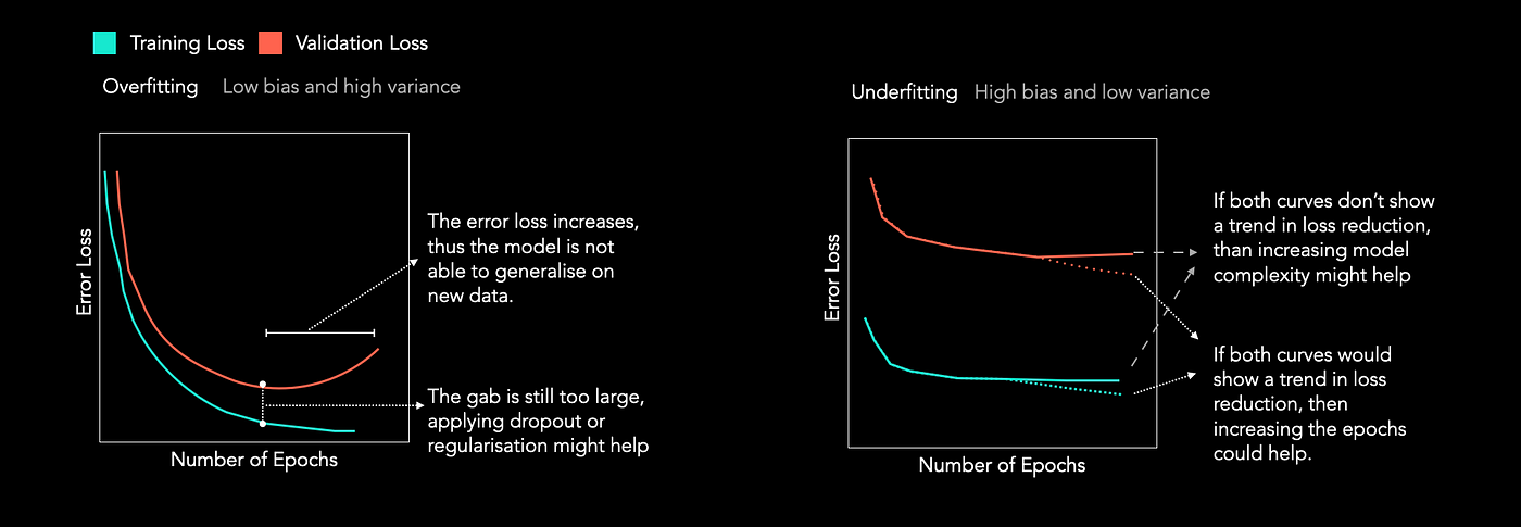
• What you see: Both the training and validation error are high and quickly plateau. There is little to no gap between them.
• What it means: The model is too simple to capture the underlying patterns in the data. It's performing poorly on the data it was trained on, and therefore, it's no surprise that it also performs poorly on new data.

Pattern 2: Overfitting (High Variance)

• What you see: The training error is low and continues to decrease. However, the validation error is significantly higher, creating a large and often growing gap between the two curves. The validation error might even start to increase after a certain point.
• What it means: The model is "memorizing" the training data, including its noise, instead of learning the generalizable signal. It becomes exceptionally good at predicting the data it has already seen, but fails when faced with new, unseen data.

Pattern 3: Good Fit (Low Bias, Low Variance)

• What you see: Both the training and validation error are low and converge to a similar value. The gap between them is small and stable.
• What it means: The model is complex enough to capture the true underlying pattern but not so complex that it starts fitting the noise. It has learned to generalize well from the training data to new data.

The following article provides a practical walkthrough with Python code, showing how to generate these three patterns by intentionally choosing different models.

To reinforce these visual patterns, here is a concise summary graphic.

3. A Formal Rule for Diagnosis

So far, we've focused on curves plotted against training epochs. A related diagnostic tool, called a validation curve, plots performance against a hyperparameter that controls model complexity (e.g., the max_depth of a decision tree or the C parameter in a Support Vector Machine).

The scikit-learn documentation provides a direct and formal rule for interpreting these plots, which perfectly summarizes today's learning objective.

The documentation provides a beautifully simple rule. It uses the term "score" (where higher is better), but the logic is the same if you're using "error" (where lower is better). Let's adapt it for both cases:

• Using a Score (e.g., Accuracy, R²):

  • If both training and validation scores are low, the model is underfitting.
  • If the training score is high and the validation score is low, the model is overfitting.

• Using an Error (e.g., MSE, RMSE):

  • If both training and validation errors are high, the model is underfitting.
  • If the training error is low and the validation error is high, the model is overfitting.

This simple comparison is one of the most fundamental diagnostic checks you will perform as a data scientist.

Conclusion

In this lesson, you have moved from defining underfitting and overfitting to actively diagnosing them by comparing training and validation performance. This is a critical skill for building models that are not only accurate on paper but also useful in the real world.

Key Takeaways:

• Plotting training and validation performance over time (or against model complexity) is a primary method for diagnosing model behavior.
• Underfitting is identified when both training and validation errors are high and plateau. The model is too simple.
• Overfitting is identified by a large and growing gap between a low training error and a high validation error. The model has memorized the training data.
• A well-fit model shows low training and validation errors that converge to similar values.

Preview of the next lesson:

Now that you can interpret these diagnostic plots, how do you create them? In the next lesson, we will focus on the practical task of plotting and interpreting learning curves using scikit-learn. You will learn how to use learning_curve to systematically evaluate how a model's performance changes as the size of the training dataset increases, providing another powerful lens to diagnose bias and variance.