Hello! Welcome back to our module on the Fundamentals of Model Validation.
In our last lesson, we learned how to look at plots of training and validation performance to conceptually diagnose underfitting and overfitting. We saw that a model performing poorly on both sets is likely underfitting, while a model that aces the training set but fails on the validation set is likely overfitting.
Today, we're going to build on that by learning how to generate and interpret one of the most powerful diagnostic tools in a data scientist's toolkit: learning curves. Your goal for this lesson is to be able to plot and interpret learning curves to diagnose bias and variance issues in your models. This will move you from simply looking at a finished chart to creating and analyzing one yourself—a key practical skill.
1. What Exactly is a Learning Curve?
In the previous lesson, we looked at performance plots versus training epochs. A classic learning curve, however, plots model performance against the size of the training set. This helps answer a critical question: "Will collecting more data actually improve my model?"
The process for generating a learning curve is systematic:
- Take a small, incremental portion of your training data.
- Train your model on this small subset.
- Evaluate the model's performance (its error or score) on both the small training subset and the entire validation set.
- Increase the size of the training subset and repeat the process.
- Finally, plot the training and validation performance against the different training set sizes.
To get a clearer picture of this process, let's turn to a great tutorial from Dataquest.
Tutorial: Learning Curves for Machine Learning in Python - Dataquest
This article, 'Learning Curves for Machine Learning in Python,' clearly explains the fundamental idea behind learning curves and how they show the relationship between training set size and model error.
Please read the section titled 'Learning curves - the basic idea'. Pay close attention to the diagram that visualizes how the training error and validation error change as the number of training instances (n) increases.
As the article explains, we typically see the training error increase as the training set grows (it's harder for the model to perfectly fit more data points), while the validation error decreases (the model generalizes better with more data). The shape and convergence of these two curves are what we will use for our diagnosis.
2. Plotting Learning Curves with Scikit-learn
Fortunately, you don't have to write the iterative process above from scratch. Scikit-learn provides a convenient learning_curve function to do the heavy lifting. This function automates the process of splitting the data into different-sized chunks, training the model, and calculating the scores using cross-validation.
Let's dive into the practical implementation.
Tutorial: Learning Curves for Machine Learning in Python - Dataquest
We'll continue with the same Dataquest article, which now shows how to use scikit-learn's learning_curve() function. This is the hands-on part you've been building towards.
Read the section 'The learning_curve() function from scikit-learn'. Focus on understanding: The key parameters of the function: estimator, X, y, train_sizes, cv, and scoring. The structure of the train_scores and validation_scores arrays it returns. Why you need to calculate the mean of the scores across the cross-validation folds before plotting.
As you saw, the learning_curve function returns arrays of scores from multiple cross-validation folds for each training set size. By averaging these scores, we get a more robust and smooth estimate of the model's performance, which is what we then plot.
3. Interpreting Learning Curves for Diagnosis
Now that you know how to generate the data for a learning curve, let's focus on interpretation. The patterns of the curves are clear indicators of bias and variance.
Let's start with a short video that beautifully illustrates the three main scenarios you'll encounter.
A Critical Skill People Learn Too LATE: Learning Curves In Machine Learning.
The video 'A Critical Skill People Learn Too LATE' from the Underfitted channel provides a quick visual guide to what underfit, overfit, and well-fit learning curves look like.
Watch from 03:14 to 06:12. Pay attention to the three distinct patterns shown: Overfitting: A large gap between training and testing loss. Well-fit: Both losses are low and close together. Two other common scenarios: a persistent gap (might need more data) and diverging test loss (trained for too long).
The video gives us a great visual intuition. Now, let's analyze these patterns in detail using the models from the Dataquest article.
Scenario 1: High Bias (Underfitting)
An underfitting model is too simple to capture the underlying patterns in the data.
- How to spot it: The training error and validation error converge to a similar, high value. There is a small gap between them.
- What it means: The model performs poorly even on the data it was trained on, and adding more data doesn't help because the model is fundamentally not complex enough to learn from it.
- What to do:
- Use a more complex model (e.g., switch from Linear Regression to a Random Forest).
- Engineer more informative features.
- Decrease regularization.
The Dataquest article provides a perfect example of this with a Linear Regression model.
Tutorial: Learning Curves for Machine Learning in Python - Dataquest
Let's examine the learning curve of a high-bias model.
Read the section 'Learning curves - high bias and low variance'. Notice how both the training and validation MSE plateau at a high value (around 20) and how the author concludes that adding more data points won't help.
Scenario 2: High Variance (Overfitting)
An overfitting model is too complex and learns the noise in the training data.
- How to spot it: There is a large and persistent gap between a low training error and a much higher validation error.
- What it means: The model has memorized the training data but fails to generalize to new, unseen data. Importantly, the validation error is often still decreasing as the training set size increases, suggesting that more data could help the model learn to generalize better.
- What to do:
- Get more training data. This is often the most effective solution.
- Increase regularization.
- Reduce model complexity (e.g., reduce the depth of a decision tree).
- Use fewer features.
The article's Random Forest example demonstrates this classic overfitting pattern.
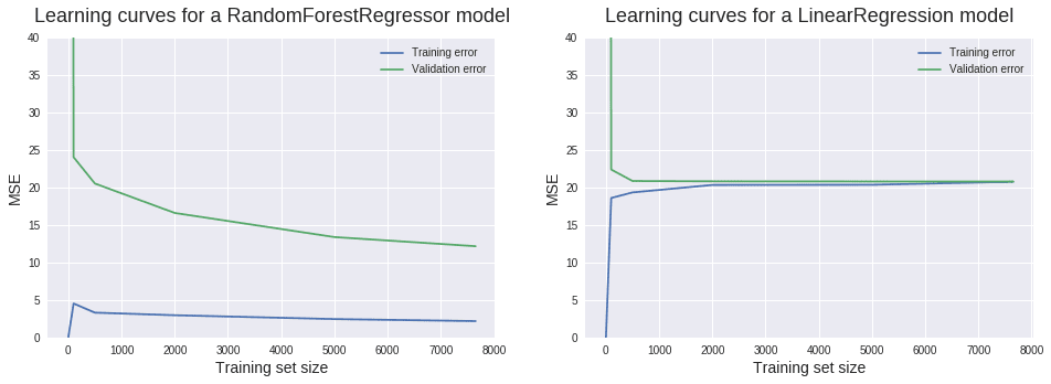
Tutorial: Learning Curves for Machine Learning in Python - Dataquest
Now, let's look at the learning curve for a high-variance model.
Read the section 'Learning curves - low bias and high variance'. Observe the large gap between the training and validation curves for the RandomForestRegressor. Note the author's conclusion: adding more training instances is likely to lead to a better model in this case.
A Note on Irreducible Error
You might wonder if the goal is to get the error to zero. In reality, this is impossible. Every dataset has some inherent amount of noise or randomness that no model can predict. This is called irreducible error. A good model's training and validation errors will converge towards this irreducible error, not towards zero. Your goal is to get the validation error as low as possible, accepting that a perfect score is unattainable.
Conclusion
In this lesson, you've taken a major step from theory to practice. You now know not just how to read a learning curve, but what it represents, how to generate one in Python, and how to use it to make concrete decisions about improving your model.
Key Takeaways:
- Learning curves plot model performance against training set size, revealing how a model's ability to learn and generalize changes with more data.
- You can generate learning curves efficiently using scikit-learn's
learning_curvefunction. - High-bias (underfitting) is diagnosed when both training and validation curves plateau at a high error. The solution is often a more complex model or better features, not more data.
- High-variance (overfitting) is diagnosed by a large gap between a low training error and a high validation error. The most common solution is to add more training data or increase regularization.
Preview of the next lesson:
So far in this module, we have built a solid foundation for diagnosing model performance. But when we say a model's error is "high" or "low," what are we comparing it to? To properly judge a model's performance, we need a benchmark. In the next lesson, we will cover how to explain the purpose of a baseline model and establish one for a given problem. This simple but essential step will provide the context needed to evaluate all your future, more complex models.