Feature Engineering: Creating New Features

1. What are Polynomial and Interaction Features?

Often, the relationship between a feature and the target variable isn't a simple straight line. For instance, the price of a house might not just increase linearly with its area; it might increase at an accelerating rate. Feature engineering allows us to capture these complex, non-linear relationships.

We'll start by exploring two techniques for this: creating polynomial features (like $x^2,x^3$) and interaction features (like $x_1\times x_2$).

To understand why we need these and how to create them, let's watch a video that starts with the limitations of a simple linear model and then introduces the solution.

As the video explained, the core idea is to transform our features. We create new columns in our dataset that are powers of the original features. Then, we can fit a LinearRegression model on this expanded set of features. The model is still linear with respect to its coefficients, but the result is a curve that can fit our data much better.

Here is a simple visual of what's happening. An original feature 'Area' is used to create a new feature 'Area^2'.

The Danger of Overfitting

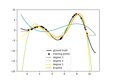
With PolynomialFeatures, you can choose the degree of the polynomial. A higher degree creates a more complex curve. While this might seem like a good thing, it comes with a significant risk: overfitting. An overly complex model might fit the noise in your training data perfectly but fail to generalize to new, unseen data. This is a key aspect of the bias-variance tradeoff you are interested in.

The next part of the video you just watched provides a great visual explanation of this risk.

This image further illustrates the concept. The goal is to find a curve that captures the underlying trend (the "ground truth") without being overly influenced by the random noise in the training points.

Interaction Features

Sometimes, the predictive power comes from the combination of two features. For example, the effectiveness of an advertising budget might depend on the season. In this case, creating a feature like ad_spend * is_holiday_season could be very powerful.

PolynomialFeatures can also create these interaction terms. The following short video explains the concept and how to create only interaction terms.

As you saw, you can generate only interaction terms by setting interaction_only=True. This is especially useful for linear models, as tree-based models like Decision Trees and Random Forests can learn interactions implicitly by how they split the data.

2. Best Practices for Implementation

Now that we have the concepts, let's look at a complete, practical implementation in Python. The best way to use PolynomialFeatures is within a scikit-learn Pipeline, which ensures your transformations are applied consistently. This also gives us a great preview of our next lesson!

This article provides a superb walkthrough and also highlights some crucial best practices.

Let's summarize the key takeaways from that reading:

• Use Pipelines: Always combine your PolynomialFeatures transformer with your model in a Pipeline. This prevents mistakes and makes your code cleaner.
• Scale Your Features First: As discussed in a previous lesson, it's critical to scale your features (e.g., using StandardScaler) before applying PolynomialFeatures. High-degree polynomials can create extremely large numbers, leading to numerical instability. The pipeline should look like: StandardScaler -> PolynomialFeatures -> LinearRegression.
• Use Cross-Validation: Don't guess the best polynomial degree. Use cross-validation to test different degrees and find the one that performs best on unseen data, not just the training data.

3. Engineering Temporal Features

Many datasets contain date and time information. In their raw format (e.g., 2023-10-27 10:30:00), these columns are not very useful for most machine learning models. We need to extract meaningful numerical features from them. This is another form of feature engineering.

Common temporal features include:

• Time elapsed between two events.
• Day of the week, month, or year.
• Time of day (e.g., morning, afternoon).
• Whether a date is a holiday.

The following resource gives practical Python examples for creating these features using pandas.

Here is a consolidated code example based on what you just read. If you have a DataFrame df with a column event_date, you can create new features like this:

import pandas as pd




# First, ensure the column is in datetime format
df['event_date'] = pd.to_datetime(df['event_date'])




# Extract date components using the .dt accessor
df['year'] = df['event_date'].dt.year
df['month'] = df['event_date'].dt.month
df['day_of_week'] = df['event_date'].dt.dayofweek # Monday=0, Sunday=6
df['hour'] = df['event_date'].dt.hour




# Calculate time elapsed since a specific point
# For example, days since the first event in the dataset
time_elapsed = (df['event_date'] - df['event_date'].min()).dt.days
df['days_since_start'] = time_elapsed

print(df.head())

This process transforms a single, unhelpful column into multiple, potentially very predictive numerical features.

Conclusion

Today, you've moved beyond data cleaning into the art of feature creation. This is a pivotal skill that separates good data scientists from great ones.

Key Takeaways:

• Feature Engineering is the process of creating new features from existing ones to improve model performance.
• Polynomial Features help models capture non-linear relationships. Use sklearn.preprocessing.PolynomialFeatures, but be cautious of overfitting by choosing the degree carefully using cross-validation.
• Interaction Features model the combined effects of two or more features. You can create them using PolynomialFeatures(interaction_only=True).
• Temporal Features are created by extracting components (like month, day of week) or calculating durations from date/time columns, typically using the pandas .dt accessor.

Preview of the next lesson:

In this lesson, you saw how a Pipeline can be used to chain a feature transformer (PolynomialFeatures) and a model. In our next session, we will fully explore this concept. You will learn how to build a reusable preprocessing pipeline using scikit-learn's Pipeline and ColumnTransformer, allowing you to combine all the steps we've learned—imputation, scaling, encoding, and feature engineering—into a single, clean, and robust object.