Outlier Handling Strategies

1. To Treat or Not to Treat? A Question of Origin

Before we jump into Python code, it's crucial to understand that handling outliers is a subjective task that requires careful consideration. The right strategy depends entirely on the source of the outlier.

To build this foundational knowledge, please read the following article. It introduces a critical distinction that will guide all of our decisions.

As you've just read, we can categorize outliers into two main types:

• Error Outliers: These are mistakes. They could be from data entry errors (e.g., a person's age entered as 200) or measurement failures. These points are not representative of the population you are studying.
• Non-Error Outliers: These are legitimate but extreme values (e.g., the salary of a CEO in a dataset of company employees). They are part of the population and can sometimes contain valuable information about the data's true variability or unique events.

This distinction directly informs our strategy:

• Error outliers should almost always be corrected (if possible) or removed.
• Non-error outliers require a more nuanced decision: we might keep them, remove them, or recode them.

2. The Main Strategies: Removal vs. Recoding

Now, let's get practical. The two most common strategies you will apply are removal (trimming) and recoding (clipping/capping). We will explore how to implement these using several popular detection methods.

This video provides an excellent hands-on walkthrough of three methods for identifying outliers and then applying both trimming and capping to handle them.

Let's consolidate what you've just seen.

Strategy 1: Removal (Trimming)

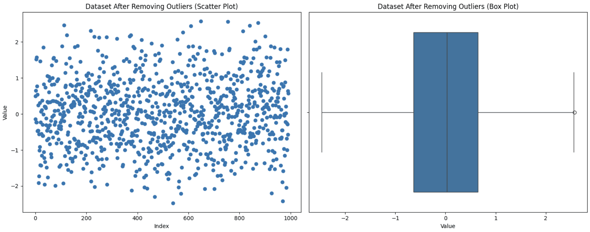
This is the most straightforward approach: you identify the outliers and simply delete the entire row from your dataset.

• When to use: Best suited for clear error outliers where you are certain the data point is invalid.
• Implementation: As shown in the video, you calculate your bounds (e.g., using IQR) and then filter the DataFrame to keep only the rows within those bounds.

# Example using the IQR method
Q1 = df['feature'].quantile(0.25)
Q3 = df['feature'].quantile(0.75)
IQR = Q3 - Q1
lower_bound = Q1 - 1.5 * IQR
upper_bound = Q3 + 1.5 * IQR




# Trimming the outliers
df_trimmed = df[(df['feature'] >= lower_bound) & (df['feature'] <= upper_bound)]

The Big Risk of Removal

While simple, removal can be dangerous. If you have many outliers or if they occur across multiple features, you could end up deleting a significant portion of your data, losing valuable information.

The next video provides a stark warning about this.

Strategy 2: Recoding (Clipping or Capping)

This is often a safer and more popular strategy. Instead of deleting the outlier, you change its value to be at a predefined upper or lower limit. This process is also known as Winsorization.

• When to use: Excellent for non-error outliers. You acknowledge the data point is extreme but reduce its ability to skew your model or analysis, all while retaining the rest of the information in that row.
• Implementation: You use the same bounds as before, but instead of filtering, you use a function like np.where() to replace values outside the bounds with the boundary values themselves.

# Example using the same IQR bounds
# Clipping the outliers
df['feature_clipped'] = np.where(df['feature'] > upper_bound, upper_bound, 
                           np.where(df['feature'] < lower_bound, lower_bound, df['feature']))

The video from Hackers Realm (resource LINK) you watched earlier demonstrated this "capping" technique for all three detection methods. It's a robust way to control extreme values without losing data records.

3. A More Advanced Approach: Imputation

For context, it's worth knowing about a more sophisticated recoding technique. This method treats outliers as missing values and then uses an imputation strategy to estimate a replacement value based on other features in the dataset. This can be very powerful but is also more complex.

The video below introduces this idea. Don't worry about mastering the code today; the goal is to understand the concept as it connects back to our earlier lessons on handling missing data.

This method is powerful because the replacement value is context-aware, but it also makes strong assumptions and requires careful implementation, including feature scaling. For now, it's an excellent concept to be aware of for future projects.

Conclusion

You've now learned the essential strategies for handling outliers, a critical step in cleaning your data for machine learning.

Key Takeaways:

• The first step is diagnosis: Is the outlier an error or a legitimate, extreme value? This determines your strategy.
• Removal (Trimming): A simple method best used for clear errors. Be very cautious, as it can lead to significant data loss.
• Recoding (Capping/Clipping): A much safer and more common approach. It reduces the influence of extreme values without deleting entire records. This is often a great default choice for non-error outliers.
• Methods for Setting Boundaries: You can define what constitutes an "outlier" using several techniques, including the Z-score (for normally distributed data), the IQR method (for skewed data), and percentiles.

Preview of the next lesson:

With our data now cleaned, scaled, and treated for outliers, we are in a great position to start creating new, more powerful predictors. In the next lesson, we will dive into Feature Engineering, where you'll learn to engineer new features from existing ones, including polynomial, interaction, and temporal features.