Visualizing Feature Distributions with Histograms and Box Plots

Introduction

Welcome to the first lesson in our module on Exploratory Data Analysis (EDA). In the previous module, we concluded by learning how to group and aggregate data to compute summary statistics like the mean or median. While these numbers are useful, they often hide the full story. For instance, two groups can have the same average value but vastly different spreads or shapes. To truly understand our data, we need to visualize its distribution.

This lesson focuses on creating two fundamental plots for this purpose: histograms and box plots. You will learn how to use Python's Matplotlib and Seaborn libraries to generate these visualizations, which are essential for understanding the distribution of individual features. This moves us from calculating single summary numbers to seeing the complete picture of a feature's spread, central tendency, and potential outliers.

Visualizing a Single Numeric Variable: The Histogram

The first tool in our visualization toolkit is the histogram. A histogram groups numbers into ranges, or "bins," and then plots the count of values falling into each bin. This immediately gives you a sense of the data's shape: Is it symmetric? Skewed to one side? Does it have one peak or multiple?

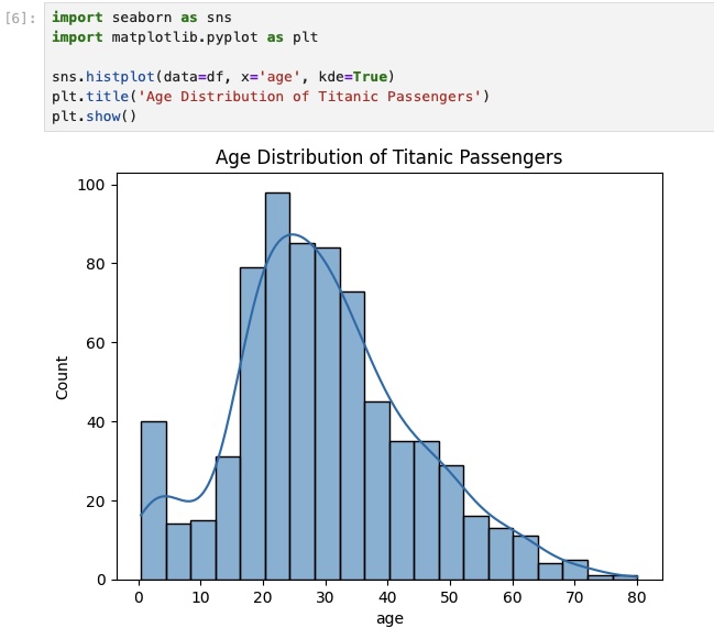
The plot below shows a typical histogram created with Seaborn. It visualizes the age distribution of Titanic passengers. We can see at a glance that the largest age group was people in their 20s and that very few passengers were over 60. The smooth line is a Kernel Density Estimate (KDE), which provides a continuous estimate of the distribution.

This histogram, generated with Seaborn, shows the distribution of passenger ages on the Titanic. The bars represent counts within specific age bins, and the curve is a Kernel Density Estimate (KDE) providing a smoothed view of the distribution.

Creating a Histogram in Python

While you can create basic histograms directly from a pandas DataFrame, the Seaborn library offers a more powerful and flexible function: sns.histplot. A recent update to Seaborn made histplot the new standard, replacing older functions.

The following video provides a concise and practical guide to using sns.histplot. It's perfect for your "how-to" learning style.

Seaborn histplot | How to make a Seaborn histogram plot with Python code

This video by Kimberly Fessel introduces the modern sns.histplot function and walks through its most important features.

Please watch the following segments: The introduction, which explains why histplot is the new standard. The basic syntax for creating a simple histogram from a pandas column. Customizing the plot, where you'll learn how to add a KDE curve and, crucially, how to control the bins using the bins, binwidth, and binrange arguments.

Controlling the number and width of bins is a key skill. Too few bins can hide important details, while too many can create a noisy, unreadable plot. Experimenting with the bins or binwidth parameter is a standard part of the analysis process.

Comparing Distributions with `hue`

A powerful feature of Seaborn is the ability to automatically split a visualization by a categorical variable using the hue argument. This lets you compare the distributions of different groups within the same plot. For example, you could compare the distribution of purchase amounts for new versus returning customers.

This next segment from the same video shows you exactly how to do this.

Seaborn histplot | How to make a Seaborn histogram plot with Python code

This section demonstrates how to use the hue parameter to create layered, stacked, or filled histograms, allowing for direct comparison of distributions across categories.

Watch the segment on splitting data by category. Pay close attention to the hue argument and the different ways to display the overlapping plots using the element and multiple arguments.

While layered histograms can be useful, they can become cluttered if you have more than two or three categories. When you need to compare many distributions at once, a box plot is often a better choice.

Summarizing and Comparing Distributions: The Box Plot

When you need a compact summary of a distribution, or when you want to compare many distributions side-by-side, the box plot is an incredibly effective tool. It displays key statistical measures in a simple visual format.

Anatomy of a Box Plot

Before creating one, it's essential to understand what a box plot represents.

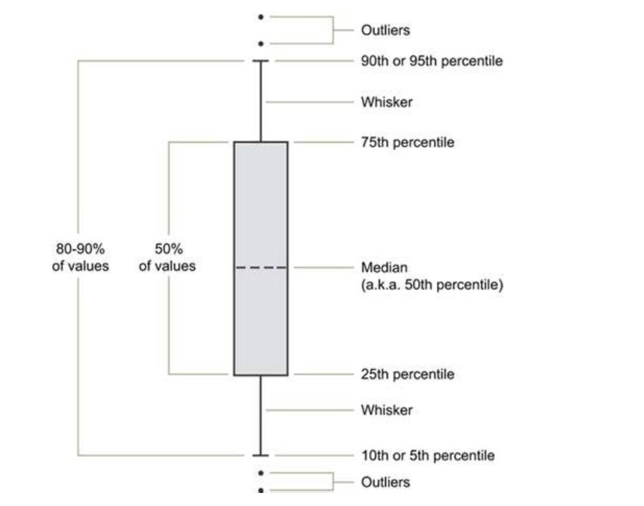
This diagram shows the components of a box plot. The box represents the Interquartile Range (IQR), containing the middle 50% of the data. The line inside is the median, the whiskers extend to show the data's range, and points beyond the whiskers are potential outliers.

The key components are:

Median (50th Percentile): The line inside the box, representing the middle value of the data.
The Box: Represents the Interquartile Range (IQR). The bottom of the box is the 25th percentile (Q1), and the top is the 75th percentile (Q3). This means the box itself contains the central 50% of your data.
Whiskers: These lines extend from the box. By default, they typically extend to 1.5 times the IQR from the top and bottom of the box. Any data points that fall outside the whiskers are plotted individually as outliers.

The video below gives a clear, practical explanation of these components and how the outlier detection rule works.

How to Make Python Boxplots with Seaborn and Matplotlib

Adam from "Analytics with Adam" provides a great walkthrough of what a box plot is and what each part signifies, including the 1.5x IQR rule for identifying outliers.

Watch the first part of the video, which gives a conceptual overview of the median, percentiles, and the structure of a box plot.

Creating Box Plots to Compare Groups

The true power of box plots shines when you use them to compare a numerical variable across different categories. This is a direct visual equivalent of the groupby() operations we performed in the last lesson. For example, you can compare the distribution of salaries across different departments or the distribution of customer satisfaction scores across different product lines.

This is a core task in practical EDA. The following resource provides an excellent, hands-on demonstration.

Python Histograms, Box Plots, & Distributions | Python Analysis Tutorial - Mode

The Mode tutorial on visualizations uses a flight delay dataset to show why box plots are superior to overlaid histograms when comparing many categories.

In the article, find the section titled Box plots. Read from this point to the end of the section. Notice how the author first tries to compare airport delays using overlaid histograms, finds it unreadable, and then switches to a box plot for a much clearer comparison. This perfectly illustrates the practical value of box plots.

While the Mode tutorial uses the pandas built-in plotting function, Seaborn's sns.boxplot offers more options and is generally preferred for creating presentation-quality plots. The next video demonstrates a complete, real-world workflow using sns.boxplot to derive business insights.

How to Make Python Boxplots with Seaborn and Matplotlib

This segment is a masterclass in practical EDA. Using a student performance dataset, the presenter shows how to use box plots to compare scores across multiple categorical variables (gender, lunch plan, test prep) and how to arrange them using subplots for a comprehensive dashboard.

This is a rich segment, so watch it carefully from applying box plots to a real dataset. Focus on these key techniques: Comparing across a single category: Creating separate box plots for "male" and "female" to compare math scores. Adding a second category with hue: Further splitting the data by "lunch plan" to see its effect on scores within each gender. Using subplots: Creating a row of plots to compare math score, reading score, and writing score all at once. This is a powerful pattern for dashboards.

This example workflow is exactly the kind of practical analysis used in professional data science settings. It moves beyond just creating a plot to using plots to ask and answer complex questions.

Conclusion

In this lesson, you've added two of the most important visualization types to your data science toolkit. You now have a practical framework for exploring the distribution of numerical data.

Here are the key takeaways:

Histograms (sns.histplot) are ideal for understanding the shape, center, and spread of a single numerical variable. Customizing the number of bins is key to getting a clear view.
Box plots (sns.boxplot) provide a compact five-number summary of a distribution (minimum, Q1, median, Q3, maximum) and are excellent for spotting outliers.
The primary strength of box plots lies in comparing distributions across many categories, a task where histograms can become cluttered.
Using parameters like hue and arranging plots in subplots allows you to build sophisticated, multi-faceted comparisons that can reveal complex patterns and lead to valuable business insights.

In our next lesson, we will move from analyzing single variables (univariate analysis) to exploring the relationships between variables. You will learn how to use scatter plots and correlation heatmaps to investigate relationships between variables, a critical step in discovering the drivers behind the trends you observe.

Recommended resources