Visualizing Relationships: Scatter Plots and Correlation Heatmaps

Welcome to your next lesson on Exploratory Data Analysis (EDA). In our previous session, we focused on univariate analysis, using histograms and box plots to understand the distribution of single variables. This was about getting to know each feature in isolation. Now, we will move on to exploring the connections between variables.

Today's lesson addresses how to investigate these relationships using two fundamental and powerful visualization techniques: scatter plots and correlation heatmaps. Mastering these will allow you to uncover patterns, dependencies, and potential drivers within your data. This is a critical step in translating raw data into actionable business insights and preparing for predictive modeling. We'll be using Python, primarily with the seaborn and pandas libraries, to create and interpret these plots.

Visualizing Relationships with Scatter Plots

When you want to understand how two numerical variables interact, the scatter plot is your primary tool. It plots each data point based on its values for two selected variables, one on the x-axis and one on the y-axis. By observing the pattern of these points, you can get a strong intuition about the relationship between the variables.

There are three main patterns you'll look for:

Positive Correlation: As the value of the x-axis variable increases, the value of the y-axis variable also tends to increase. The points will trend upwards from left to right.
Negative Correlation: As the x-axis variable increases, the y-axis variable tends to decrease. The points will trend downwards from left to right.
No Correlation: There is no discernible pattern. The points are scattered randomly.

For a clear explanation of these concepts and how to create scatter plots in Python, the following resource is an excellent starting point.

Exploratory Data Analysis with Python: An Overview

This article provides a concise overview of different EDA techniques. We'll focus on the section covering scatter plots.

Please read the section under the heading Scatter Plot. It introduces the concept, provides sample code for creating basic and enhanced scatter plots, and discusses how to interpret different types of correlations visually.

To see these concepts applied in a live coding session, the following video demonstrates the process with a dataset of roller coaster statistics. Pay close attention to how a third variable is introduced using color, a technique that significantly enhances the plot's informational density.

Exploratory Data Analysis with Pandas Python

This video by Rob Mulla provides a practical walkthrough of creating various plots for EDA.

Watch the segment on feature relationships. The first part uses pandas' built-in plotting, but the more important part starts at the transition to seaborn. Notice how the hue parameter is used to add the 'year introduced' as a third dimension to the scatter plot.

The basic syntax for a scatter plot in seaborn is straightforward:

import seaborn as sns
import matplotlib.pyplot as plt




# Assuming 'df' is your pandas DataFrame
sns.scatterplot(data=df, x='your_x_variable', y='your_y_variable')
plt.title('Relationship between X and Y')
plt.show()

To add a third, categorical variable, you simply add the hue parameter:

sns.scatterplot(data=df, x='your_x_variable', y='your_y_variable', hue='your_categorical_variable')
plt.title('Relationship between X and Y, segmented by Category')
plt.show()

Quantifying Relationships with Correlation

While scatter plots give us a visual sense of a relationship, the correlation coefficient provides a numerical measure of the strength and direction of a linear relationship between two variables. The most common is the Pearson correlation coefficient, denoted as r.

r = +1: Perfect positive linear relationship.
r = -1: Perfect negative linear relationship.
r = 0: No linear relationship.

Values between 0 and 1 (or 0 and -1) indicate the strength of the relationship. For instance, r = 0.8 signifies a strong positive linear correlation, while r = -0.2 signifies a weak negative linear correlation.

It's crucial to remember that correlation only measures linear relationships. A perfect non-linear relationship (e.g., a parabola) might have a correlation coefficient of 0. This is why visualizing your data with a scatter plot first is so important.

In Python, you can easily calculate the correlation matrix for all numerical columns in a DataFrame using the .corr() method in pandas.




# Assuming 'df_numeric' contains only the numerical columns of your DataFrame
correlation_matrix = df_numeric.corr()
print(correlation_matrix)

Visualizing the Correlation Matrix with a Heatmap

A table of correlation numbers can be difficult to interpret, especially with many variables. A heatmap solves this by representing the correlation matrix visually, using color to denote the strength and direction of the correlation. This allows you to spot significant relationships at a glance.

The following guide and video provide a complete walkthrough, from calculating the correlation matrix to visualizing it as an annotated heatmap.

7. Correlation and Scatterplots — Basic Analytics in Python

This resource offers a step-by-step guide to calculating and visualizing correlations.

Focus on the sections Corrleation matrix to see how to generate the matrix with pandas, and Correlation matrix to heat map, which explains how to turn that matrix into a heatmap with seaborn.

For a detailed demonstration, the next video walks through this exact process on a real dataset.

Exploratory Data Analysis Step-by-Step Walkthrough | Python Pandas Tutorial | Data Science Tutorial

This step-by-step tutorial provides excellent, clear instructions for creating and interpreting a correlation heatmap.

Please watch the section on multivariate analysis. The presenter demonstrates how to: Isolate numerical columns for the correlation calculation. Compute the correlation matrix with .corr(). Create a heatmap using seaborn.heatmap(). Add annotations (annot=True) and a custom color map (cmap) to make the plot easy to read.

Here is the Python code to generate an annotated heatmap:




# First, compute the correlation matrix
correlation_matrix = df_numeric.corr()




# Then, create the heatmap
plt.figure(figsize=(12, 10)) # Adjust size as needed
sns.heatmap(correlation_matrix, annot=True, cmap='coolwarm', fmt='.2f')
plt.title('Correlation Heatmap of Features')
plt.show()

annot=True displays the correlation coefficient in each cell.
cmap='coolwarm' uses a color scheme where warm colors (red) indicate positive correlation and cool colors (blue) indicate negative correlation.
fmt='.2f' formats the annotations to two decimal places.

Interpreting a Business-Focused Heatmap

Let's apply this to a practical example. Below is a correlation heatmap for various metrics from an eCommerce store.

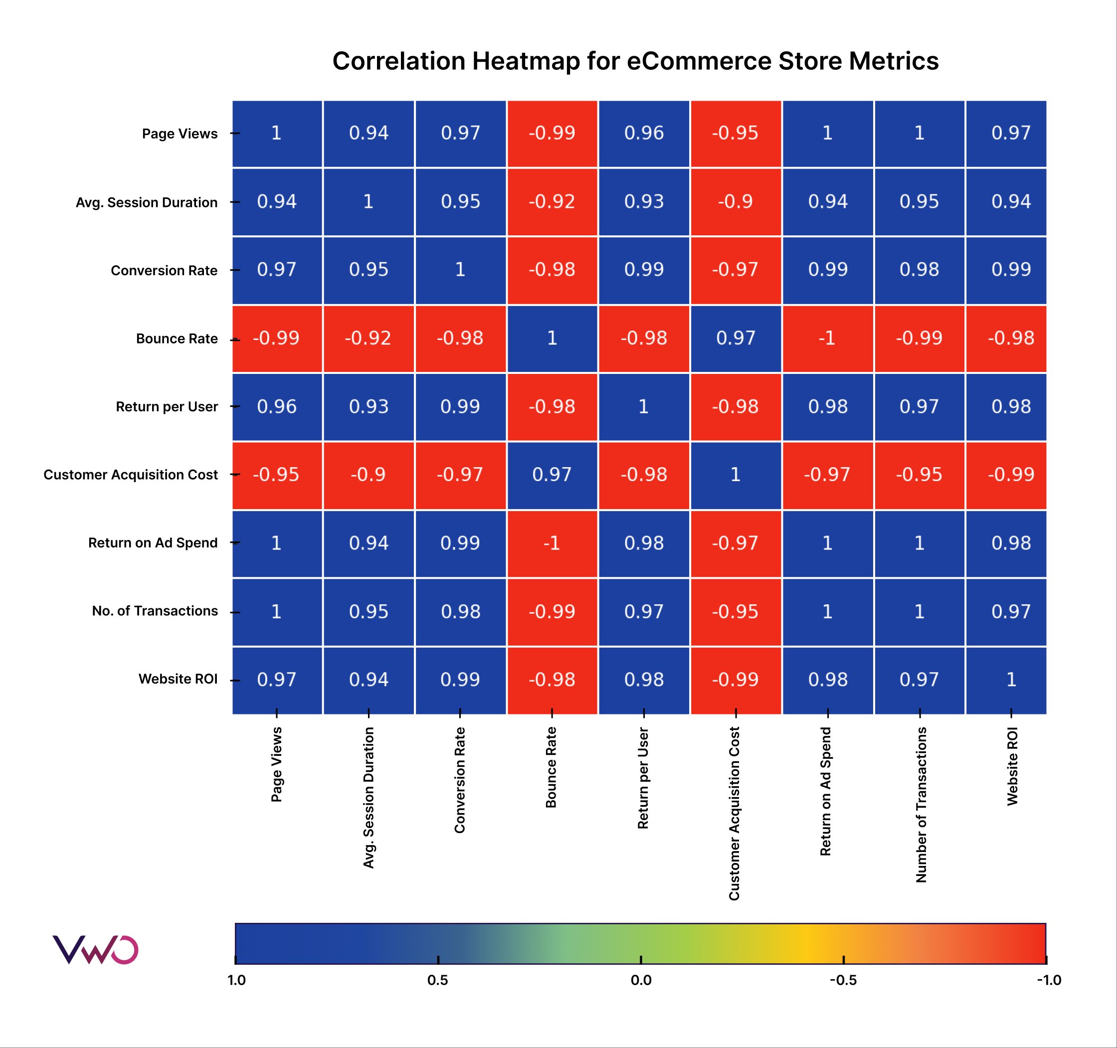
A correlation heatmap showing the relationships between key performance indicators for an online store. Red indicates a strong negative correlation, blue indicates a strong positive correlation, and white/yellow indicates a weak or no correlation.

Take a moment to analyze the chart and consider these questions:

What is the relationship between Conversion Rate and Bounce Rate? What does a correlation of -0.98 tell you about user behavior on the site?
Look at the correlation between Customer Acquisition Cost (CAC) and Website ROI. Does the relationship make business sense? Why?
Identify two variables that have a very strong positive correlation (close to 1). Why might these two metrics be so closely related?

This exercise of translating the numerical values and colors into a business narrative is precisely the goal of this type of analysis.

A Powerful Shortcut: The Pair Plot

What if you want to quickly see all the scatter plots and distributions for multiple variables at once? Seaborn offers a fantastic function for this: pairplot(). It creates a matrix of plots, showing a scatter plot for every pair of variables and a histogram or density plot for each variable on the diagonal.

This cheatsheet shows a pair plot under "Multivariate Analysis," demonstrating how it combines scatter plots and histograms to analyze numerical variables.

The pairplot is an incredibly efficient way to get a rapid overview of your dataset. You can even add a hue argument to segment the data by a categorical variable, just like with a scatter plot.




# Creates scatter plots for every pair of columns and histograms on the diagonal
sns.pairplot(df_numeric)
plt.show()




# You can also add a categorical variable for color-coding
sns.pairplot(df, hue='your_categorical_variable')
plt.show()

Key Takeaways

In this lesson, you've learned to move from single-variable to multi-variable analysis. Here are the main points:

Scatter plots are used to visually inspect the relationship between two numerical variables, revealing patterns like positive, negative, or no correlation.
The correlation coefficient quantifies the strength and direction of a linear relationship, with pandas.DataFrame.corr() being the primary tool for calculation.
Correlation heatmaps, created with seaborn.heatmap(), provide a powerful, high-level view of the linear relationships across all numerical features in your dataset.
Pair plots offer a quick way to generate scatter plots and histograms for multiple variables simultaneously, making them an excellent first step in multivariate exploration.

These techniques are fundamental to EDA. By identifying which variables are related, you can begin to form hypotheses about what drives the outcomes you care about—a key step before building any predictive models.

In our next lesson, we will focus on detecting and analyzing outliers. The scatter plots and box plots you now know how to create will be your essential tools for spotting these unusual data points.