Hello! Welcome to the fifth lesson in our "Deep Learning Foundations" module.
In our previous lesson, we explored how optimizers like SGD and Adam use the gradients calculated during backpropagation to update a model's weights. We now have a complete training loop: we can feed data to our model, calculate its error, and use an optimizer to nudge its parameters in the right direction, repeating this process over many epochs.
But as we train, a crucial question arises: Is the model actually learning to generalize, or is it just memorizing the training data? A model that only memorizes is useless on new, unseen data.
Today, you will learn how to become a "model diagnostician." We'll explore two of the most fundamental concepts in machine learning—overfitting and underfitting—and you'll learn how to diagnose these conditions by plotting and interpreting learning curves. This is one of the most critical skills for any machine learning practitioner.
1. The Challenge of Generalization
The goal of training a model is not to achieve perfect performance on the training data. The true goal is generalization: the ability to make accurate predictions on new data it has never seen before.
Two common failure modes prevent good generalization:
- Underfitting: The model is too simple to capture the underlying patterns in the data. It fails to learn effectively.
- Overfitting: The model is so complex that it learns the training data perfectly, including the noise and random fluctuations. It essentially memorizes the training set and fails to generalize to new data.
Let's start with a video that provides an excellent analogy to understand these concepts.
A Critical Skill People Learn Too LATE: Learning Curves In Machine Learning.
This video from the 'Underfitted' channel uses a clear analogy of a student preparing for an exam to explain underfitting and overfitting. It then introduces learning curves as the primary tool for diagnosing them.
Watch the first two minutes of the video (00:00 - 02:01). Focus on the connection between a student 'learning the material' vs. 'optimizing for the exam' and how this relates to a model's ability to generalize.
2. What are Learning Curves?
As the video introduced, our primary diagnostic tool is the learning curve. A learning curve is a plot showing a model's performance over time (typically measured in epochs).
To create a meaningful learning curve, we plot two lines:
- Training Loss/Metric: The model's performance on the data it is being trained on. This tells us how well the model is "learning."
- Validation Loss/Metric: The model's performance on a separate, held-out validation set. This data is not used for training and serves as a proxy for unseen, real-world data. This tells us how well the model is "generalizing."
By comparing these two curves, we can gain deep insights into our model's behavior.
Let's dive into a comprehensive resource that defines the classic patterns you'll see in learning curves.
How to use Learning Curves to Diagnose Machine Learning Model Performance
This article from Machine Learning Mastery is a classic reference for interpreting learning curves. It provides clear definitions and example plots for underfitting, overfitting, and a good fit.
Read the section titled 'Diagnosing Model Behavior', including its three subsections: 'Underfit Learning Curves', 'Overfit Learning Curves', and 'Good Fit Learning Curves'. For each one, study the text description and the corresponding example plot.
3. Interpreting the Patterns
Based on the article you just read, let's summarize the key patterns.
Underfitting
An underfit model fails to capture the complexity of the data.
- Symptom: The model performs poorly on both the training and validation sets.
- Learning Curve:
- Training loss and validation loss are both high.
- The curves plateau at a high loss value, showing the model is unable to learn further.
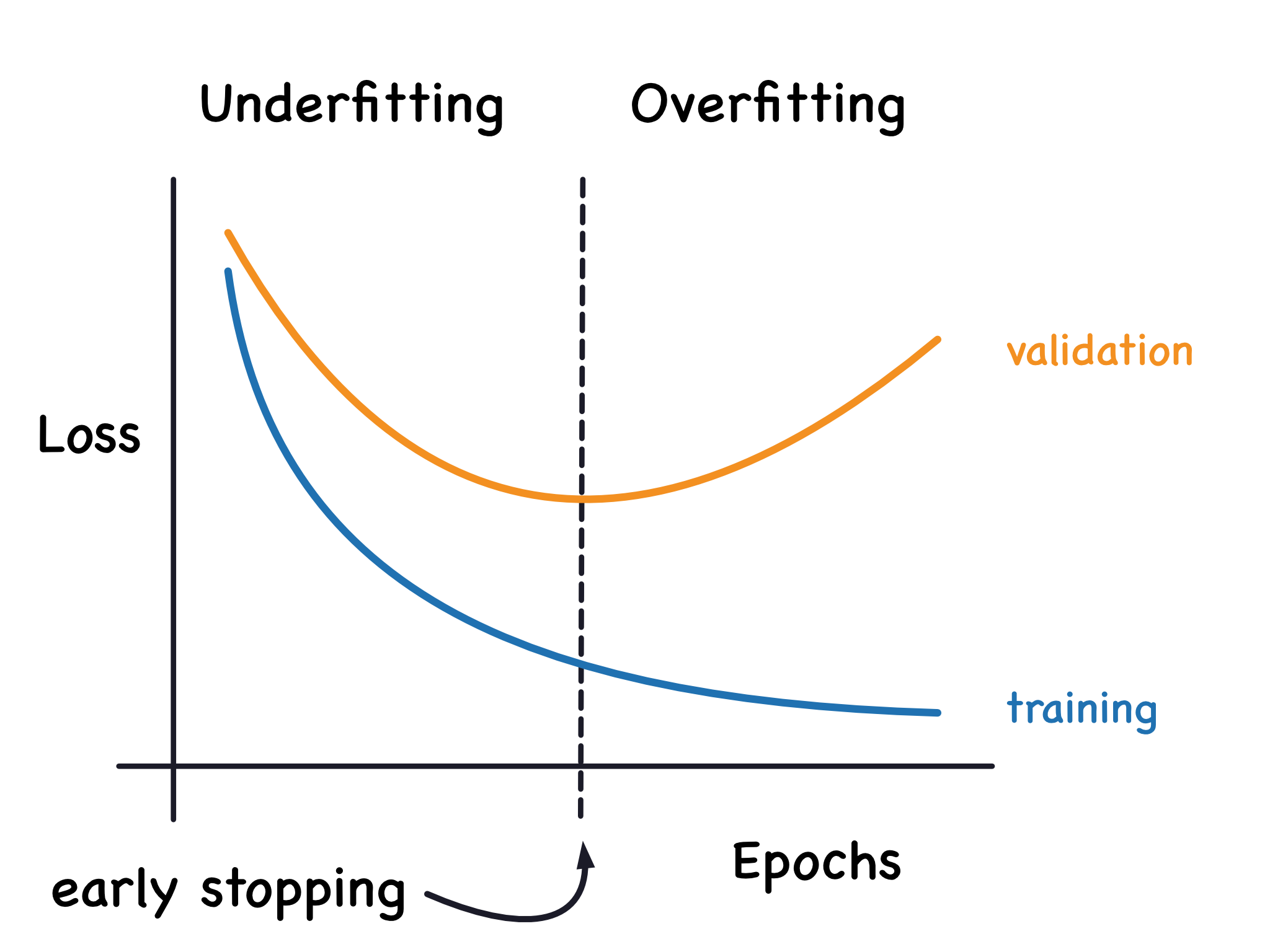
Overfitting
An overfit model has learned the training data too well, including its noise.
- Symptom: The model performs exceptionally well on the training data but poorly on the validation data.
- Learning Curve:
- Training loss continues to decrease to a very low value.
- Validation loss decreases for a while, but then begins to increase.
- A significant and widening gap appears between the training and validation curves.
Good Fit
A well-fit model has learned the true underlying pattern in the data.
- Symptom: The model performs well on both the training and validation sets.
- Learning Curve:
- Both training and validation loss decrease and converge to a low, stable value.
- There is a small, stable gap between the two curves (this is the "generalization gap"). It's normal for validation loss to be slightly higher than training loss.
4. A Practical PyTorch Example
Now, let's see how to generate and visualize these curves in code. We'll use a practical example where we deliberately create a complex model to observe overfitting.
The resource below walks through a complete PyTorch example:
- Generates synthetic data (a sine wave with noise).
- Defines two models: a simple one and a complex one (which is prone to overfitting).
- Implements a training loop that tracks training and validation loss at each epoch.
- Plots the resulting learning curves to diagnose the model's behavior.
This is a perfect hands-on exercise to solidify your understanding.
Practice: Visualizing Overfitting
The article 'Practice: Visualizing Overfitting' from ApX Machine Learning provides a complete, runnable PyTorch code example to demonstrate overfitting. It's an excellent way to connect the theory to practical implementation.
Read through this entire article. Pay close attention to the code blocks and the explanations. Understand the setup: See how synthetic data is created and split. Compare the models: Notice the difference in architecture between SimpleModel and ComplexModel. The ComplexModel has much more capacity. Analyze the training loop: The train_model function is key. See how train_losses and val_losses are appended at each epoch. Interpret the results: Examine the learning curve plots and the model prediction plots. See how the complex model's curve shows a clear overfitting pattern, and its prediction plot wiggles to catch the noise in the training data.
After working through that example, you should have a clear mental model:
- Model Capacity is Key: A model with high capacity (many layers/neurons) is more likely to overfit a simple dataset.
- Tracking Loss is Simple: The core logic involves storing the training and validation loss from each epoch in lists and then plotting them using Matplotlib.
5. Interpreting More "Noisy" Real-World Curves
The examples we've seen so far are quite clean. In real projects, learning curves can be more complex and noisy. The next video shows a variety of learning curves generated by training models of different complexities on a real dataset.
154 - Understanding the training and validation loss curves
This video from DigitalSreeni provides a fantastic practical walkthrough. The presenter trains models of increasing complexity on the Wisconsin breast cancer dataset and analyzes the resulting 'messy' learning curves, giving you a taste of what you'll encounter in practice.
Watch the sections analyzing the results of different models: Dense 16 (Good Fit): Watch from 16:37 to 18:36. This is a great example of what a good, well-behaved learning curve looks like. Two Dense Layers (Overfitting): Watch from 18:36 to 20:10. Here, you'll see a classic overfitting pattern emerge as the model becomes more complex. Six Dense Layers (Severe Overfitting): Watch from 20:10 to 21:30. This demonstrates how a model that is far too complex for the dataset produces dramatic overfitting. Summary: Finally, watch the summary from 23:18 to 27:11, where he recaps the visual characteristics of underfitting, overfitting, and a good fit.
One interesting point raised in the video is that sometimes validation loss can be lower than training loss. This might seem counter-intuitive, but it can happen for a few reasons:
- Regularization: Techniques like Dropout (which we'll cover in the next lesson) are applied during training but not during validation, making the training task harder for the model.
- Unrepresentative Sets: The validation set might happen to be "easier" than the training set due to a random, unlucky data split.
Conclusion
You now have a powerful diagnostic framework for understanding your model's training behavior. By plotting and analyzing training and validation learning curves, you can confidently determine if your model is underfitting, overfitting, or achieving a good fit.
Key Takeaways:
- Learning Curves plot training and validation performance (e.g., loss) against epochs to diagnose model behavior.
- Underfitting is identified by high loss on both training and validation sets. The model is too simple.
- Overfitting is identified by a low training loss but a high and increasing validation loss. The model has memorized the training data.
- A Good Fit is identified when both training and validation loss converge to a low value with a small, stable gap between them.
- Plotting these curves in PyTorch involves saving the loss from each epoch in a list and then using a plotting library like Matplotlib.
Preview of the Next Lesson:
We've spent this lesson learning how to diagnose the problem of overfitting. The natural next question is: "How do we fix it?" In our next lesson, "Apply regularization techniques: dropout and batch normalization," we will explore powerful techniques designed specifically to combat overfitting and help your models generalize better.