SGD and Adam Optimizers for Neural Networks

1. The Role of an Optimizer

An optimizer is the algorithm that implements the gradient descent strategy. Its job is to take the gradients calculated during backpropagation and use them to update the network's weights and biases in a way that minimizes the loss function.

The simplest form of this update rule is:

Here, $\eta$ (eta) is the learning rate, a small positive number that controls the size of the update step. In the previous lesson, we saw how loss.backward() calculates the gradient. The optimizer is responsible for performing this update step across all parameters.

Let's begin with a video that recaps the training process and introduces the most fundamental optimizer: Stochastic Gradient Descent (SGD).

As the video explains, Stochastic Gradient Descent (SGD) performs this update for each parameter using the gradient calculated from a small batch of training data (a "mini-batch"). While simple and effective, "vanilla" SGD has some significant challenges:

• It can be slow to converge if the loss landscape is like a long, narrow ravine.
• It can get stuck in local minima (small valleys that aren't the lowest point).
• The update steps can be very noisy and erratic.

To address these issues, more advanced optimizers were developed.

2. Enhancing SGD: Momentum and Adaptive Learning Rates

Modern optimizers build upon SGD by incorporating more sophisticated techniques. Two key ideas are momentum and adaptive learning rates.

Momentum: Gathering Speed

Imagine a ball rolling down a hilly landscape. Instead of stopping at every point to check the steepest direction, it builds up momentum, helping it to roll over small bumps and accelerate down long slopes.

The momentum technique in optimization applies the same intuition. It calculates the weight update using an exponentially weighted average of past gradients. If the gradients have been consistently pointing in the same direction, the "velocity" in that direction increases, leading to larger update steps.

This helps in two ways:

1. Speeds up convergence, especially in long, narrow "ravines" in the loss landscape.
2. Helps escape local minima by allowing the optimizer to "roll over" small humps.

Let's see a visual explanation of momentum.

Adaptive Learning Rates: Different Steps for Different Parameters

In a typical neural network, some parameters might have very steep gradients, while others have very gentle ones. Using a single learning rate for all parameters can be inefficient.

• A large learning rate might cause the optimizer to overshoot the minimum for parameters with steep gradients.
• A small learning rate might cause very slow progress for parameters with gentle gradients.

Adaptive learning rate methods solve this by giving each parameter its own learning rate, which is adjusted during training. A popular algorithm that introduced this idea is RMSprop (Root Mean Square Propagation). It keeps track of the squared gradients for each parameter and scales its learning rate inversely to this magnitude. In simple terms:

• If a parameter has large gradients, its effective learning rate is reduced.
• If a parameter has small gradients, its effective learning rate is increased.

This helps to balance the learning process across all parameters.

3. Adam: Combining Momentum and Adaptive Learning Rates

So, what happens if we combine the ideas of momentum and adaptive learning rates? We get the Adam (Adaptive Moment Estimation) optimizer.

Adam is one of the most popular and effective optimizers in deep learning. It computes adaptive learning rates for each parameter (like RMSprop) and also keeps track of an exponentially weighted average of past gradients (like momentum).

Let's see Adam in action and then dive into its mechanics.

To solidify your understanding of Adam's equations, Andrew Ng provides a clear, step-by-step breakdown. Given your interest in the mathematical foundations, this will be a valuable watch.

4. Using Optimizers in PyTorch

The great news is that you don't have to implement these complex algorithms from scratch. PyTorch provides them in its torch.optim module.

The standard training loop in PyTorch, which connects backpropagation with the optimizer, looks like this:

1. optimizer.zero_grad(): Clear old gradients from the previous step.
2. outputs = model(inputs): Perform the forward pass to get predictions.
3. loss = criterion(outputs, labels): Calculate the loss.
4. loss.backward(): Perform backpropagation to compute gradients for all parameters.
5. optimizer.step(): The optimizer updates all parameters using the computed gradients.

Here is how you would initialize SGD and Adam optimizers in PyTorch:

import torch
import torch.optim as optim




# Assume `model` is your nn.Module instance
# Initialize SGD optimizer
optimizer_sgd = optim.SGD(model.parameters(), lr=0.01, momentum=0.9)




# Initialize Adam optimizer
optimizer_adam = optim.Adam(model.parameters(), lr=0.001) 



# Note: Adam often uses a smaller learning rate than SGD




# Inside your training loop for each batch:
optimizer_adam.zero_grad()



# ... forward pass ...
# ... calculate loss ...
loss.backward()
optimizer_adam.step()

Notice that we pass model.parameters() to the optimizer. This tells the optimizer which tensors (weights and biases) it is responsible for updating. The lr (learning rate) is the most important hyperparameter to tune.

For a practical guide on how to set this up, the following resource is very helpful.

5. Which Optimizer Should You Use?

Adam's combination of momentum and adaptive learning rates makes it very powerful. It often converges much faster and is less sensitive to the choice of learning rate than SGD. For most problems, Adam is an excellent default choice.

The following charts visually demonstrate Adam's superior performance in many common scenarios.

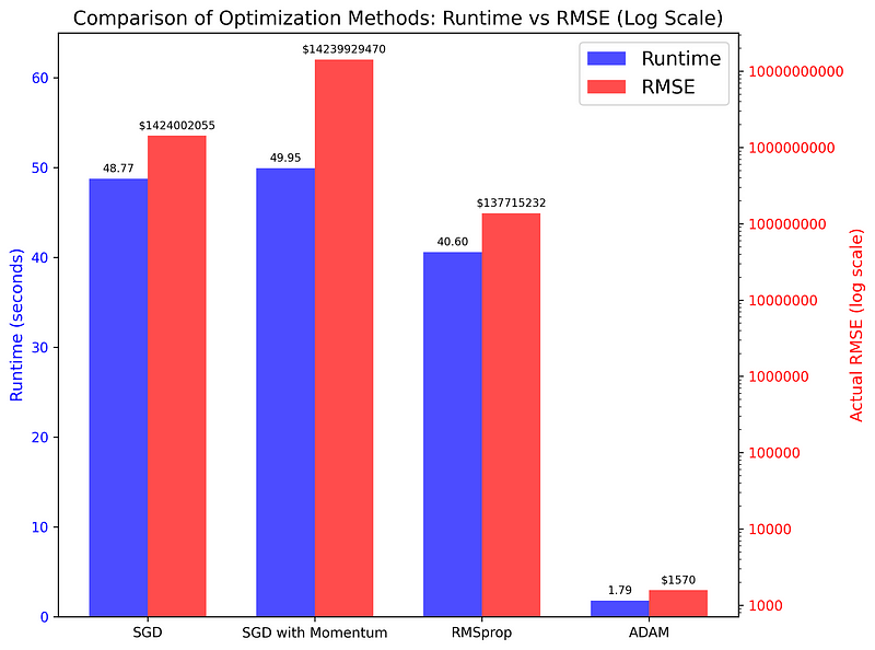
However, the choice is not always so simple. Some research suggests that while Adam is faster, models trained with SGD (especially with momentum) can sometimes generalize better to unseen data. This is thought to be because SGD may find "wider" minima in the loss landscape, which are more robust.

To explore this nuance further, let's look at a resource that visualizes how different optimizers behave on tricky loss surfaces.

Conclusion

You have now connected the dots from calculating gradients to actually training a model. You are equipped with the knowledge to drive the learning process of any neural network.

Key Takeaways:

• Optimizers are algorithms that use gradients from backpropagation to update model weights and minimize loss.
• Stochastic Gradient Descent (SGD) is the foundational optimizer, but it can be slow and unstable.
• Momentum helps accelerate training and navigate difficult loss surfaces by incorporating past gradients.
• Adaptive Learning Rates (used in RMSprop and Adam) adjust the step size for each parameter individually, leading to more efficient training.
• Adam (Adaptive Moment Estimation) combines both momentum and adaptive learning rates, making it a powerful and widely used default choice.
• In PyTorch, you can easily use these optimizers via the torch.optim module within a standard training loop (zero_grad, backward, step).

Preview of the Next Lesson:
We now know how to run a full training loop over many epochs. But how do we know if the training is going well? How can we tell if the model is actually learning or just memorizing the training data? In our next lesson, "Diagnose overfitting and underfitting using learning curves," you will learn how to monitor your model's training process by plotting performance metrics over time to gain crucial insights.