Backpropagation and Gradient Descent

1. The Goal: Minimizing Error with Gradient Descent

Before we dive into how a network learns, let's clarify what it's trying to achieve. The goal is to adjust the model's parameters (weights and biases) so that its predictions get progressively closer to the actual target values in the training data.

To do this, we first need a way to measure how "wrong" the model's current predictions are. This is done using a cost function (or loss function). A common example is the Mean Squared Error (MSE), which we saw briefly in the mathematics module:

The cost is a single number that summarizes the model's performance. A high cost means bad predictions; a low cost means good predictions. Our goal is to find the set of weights and biases that results in the lowest possible cost.

This is an optimization problem. The most common way to solve it in deep learning is gradient descent. Imagine the cost function as a vast, hilly landscape where your position is determined by the current values of the network's weights. The altitude at your position is the cost. To minimize the cost, you need to find the lowest valley.

The gradient ($\nabla C$) is a vector of partial derivatives that points in the direction of the steepest ascent from your current position. To go downhill, you simply take a small step in the opposite direction of the gradient. You repeat this process, and eventually, you will arrive at a local minimum of the cost function.

The core challenge is calculating this gradient, which consists of the partial derivative of the cost with respect to every single weight and bias in the network. For a model with millions of parameters, this seems like a monumental task. This is where backpropagation comes in.

2. Backpropagation: The Chain Rule in Action

Backpropagation is an algorithm that efficiently computes the gradient of the cost function. It works by first running a forward pass to compute the output and the cost, and then propagating the error signal backward through the network to calculate how much each parameter contributed to that error.

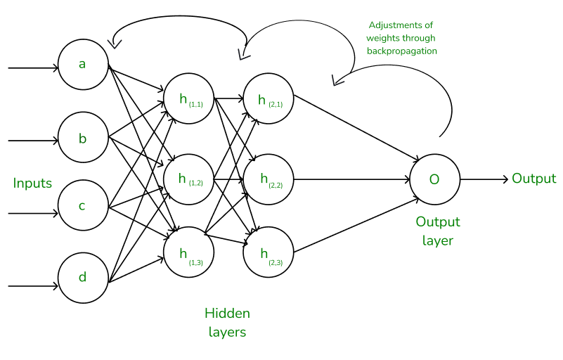
The mathematical heart of backpropagation is the chain rule from calculus. Let's see how it works.

The following video from 3Blue1Brown provides one of the best explanations of the calculus behind backpropagation. It masterfully connects the abstract math to the structure of a neural network.

As the video explains, for a single weight $w^{(L)}$ in the final layer, the gradient is calculated by chaining together derivatives:

Let's break down these three parts:

1. $\frac{\partial z^{(L)}}{\partial w^{(L)}}=a^{(L-1)}$: The effect of the weight on the neuron's pre-activation sum $z$ depends on the activation of the neuron from the previous layer. This is the "neurons that fire together, wire together" principle in mathematical form.
2. $\frac{\partial a^{(L)}}{\partial z^{(L)}}={\sigma }^{\prime }(z^{(L)})$: The effect of the pre-activation sum on the final activation depends on the slope of the activation function at that point.
3. $\frac{\partial C}{\partial a^{(L)}}=2(a^{(L)}-y)$: The effect of the final activation on the cost is proportional to the error itself. If the prediction is far from the actual value, this term will be large.

Backpropagation simply organizes these chain rule calculations, starting from the cost and working backward through the layers, reusing computations along the way to remain efficient.

3. A Step-by-Step Numerical Example

The theory and the formulas can feel abstract. To make it concrete, let's walk through a numerical example. The following video provides a clear, step-by-step calculation of backpropagation for a small network.

If you prefer a text-based walkthrough with all the equations laid out, the following article is an excellent alternative. It meticulously details the same process.

By working through these examples, you can see how the abstract concept of the chain rule becomes a concrete algorithm for computing the exact adjustments needed for each weight and bias in the network.

4. Backpropagation in PyTorch: autograd

Understanding the mechanics of backpropagation is crucial for any deep learning practitioner. However, the good news is that you will rarely, if ever, have to implement it by hand. Modern deep learning frameworks like PyTorch automate this entire process with a system called automatic differentiation, or autograd.

Here’s how it works:

1. When you perform the forward pass using PyTorch tensors (where requires_grad=True), PyTorch builds a computational graph. This graph records every operation that was performed to get from the input to the final cost.
2. When you call loss.backward(), PyTorch's autograd engine traverses this graph in reverse.
3. At each step, it applies the chain rule to compute the gradients for all the parameters that were involved in the computation.
4. These gradients are then stored in the .grad attribute of each parameter tensor (e.g., model.layer1.weight.grad).

This powerful feature is why we use frameworks. It allows us to define complex architectures while the framework handles the intricate calculus of gradient computation behind the scenes.

Conclusion

You have now uncovered the core learning mechanism of neural networks. While we defined the structure of a network in the last lesson, today you learned about the process that brings it to life.

Key Takeaways:

• Neural networks learn by minimizing a cost function using an optimization algorithm like gradient descent.
• Gradient descent requires the gradient of the cost function with respect to all model parameters (weights and biases).
• Backpropagation is an efficient algorithm that uses the chain rule to compute this gradient by propagating error signals backward from the output layer.
• The calculated gradient tells us the direction and magnitude of the change needed for each parameter to reduce the cost.
• In PyTorch, the autograd engine automatically computes these gradients when you call .backward() on the loss tensor.

Preview of the Next Lesson:
We now have the "direction" to step in to reduce our model's error. But how large of a step should we take? How do we use the gradients to update the weights? In the next lesson, "Train neural networks using SGD and Adam optimizers," we will explore the algorithms that perform these updates and drive the training loop.