Hello! Welcome to the second lesson in our Natural Language Processing module.
In our last lesson, we learned how to perform essential text preprocessing steps—tokenization, stopword removal, and lemmatization—to transform raw text into a clean list of meaningful words (tokens). However, machine learning algorithms don't understand words; they understand numbers.
This lesson bridges that gap. Your learning outcome is to represent text using Bag-of-Words and TF-IDF vectors. We will explore two fundamental techniques that convert your cleaned tokens into numerical feature vectors, making them ready for machine learning models. This process is a cornerstone of classical NLP and a crucial step in building many language-based applications.
1. Why Convert Text to Numbers?
Before we dive into the "how," let's solidify the "why." Machine learning models are mathematical functions. They operate on numerical data arranged in vectors and matrices. How can we represent something as abstract as a sentence in this numerical format?
Unlike images, which are inherently grids of pixel values, or audio, which can be represented as a series of amplitude values, text doesn't have an obvious numerical equivalent. We need to create a system to encode the information contained in words into numbers.
This first video explains this challenge and sets the stage for the vectorization techniques we'll learn today.
Text Representation | NLP Lecture 4 | Bag of Words | Tf-Idf | N-grams, Bi-grams and Uni-grams
Let's watch a segment from the video "Text Representation | NLP Lecture 4" by CampusX. It does an excellent job of explaining why text requires a different approach to numerical conversion compared to other data types like images or audio.
Watch from 02:54 to 12:02. Focus on the core problem: machine learning algorithms need numbers. Pay attention to the comparison between representing images, audio, and text, and the key goal of capturing the 'semantic meaning' of the text in the numerical representation.
2. Method 1: The Bag-of-Words (BoW) Model
The simplest and most intuitive way to represent text numerically is the Bag-of-Words (BoW) model.
The core idea is to treat each document as an unordered collection—a "bag"—of its words. We disregard grammar and word order and focus only on whether a word is present and how many times it appears.
Here's the process:
- Build a Vocabulary: Collect every unique word from our entire collection of documents (the corpus).
- Vectorize: For each document, create a vector that has the same length as our vocabulary. Each position in the vector corresponds to a unique word. The value at that position is the count of how many times that word appears in the document.
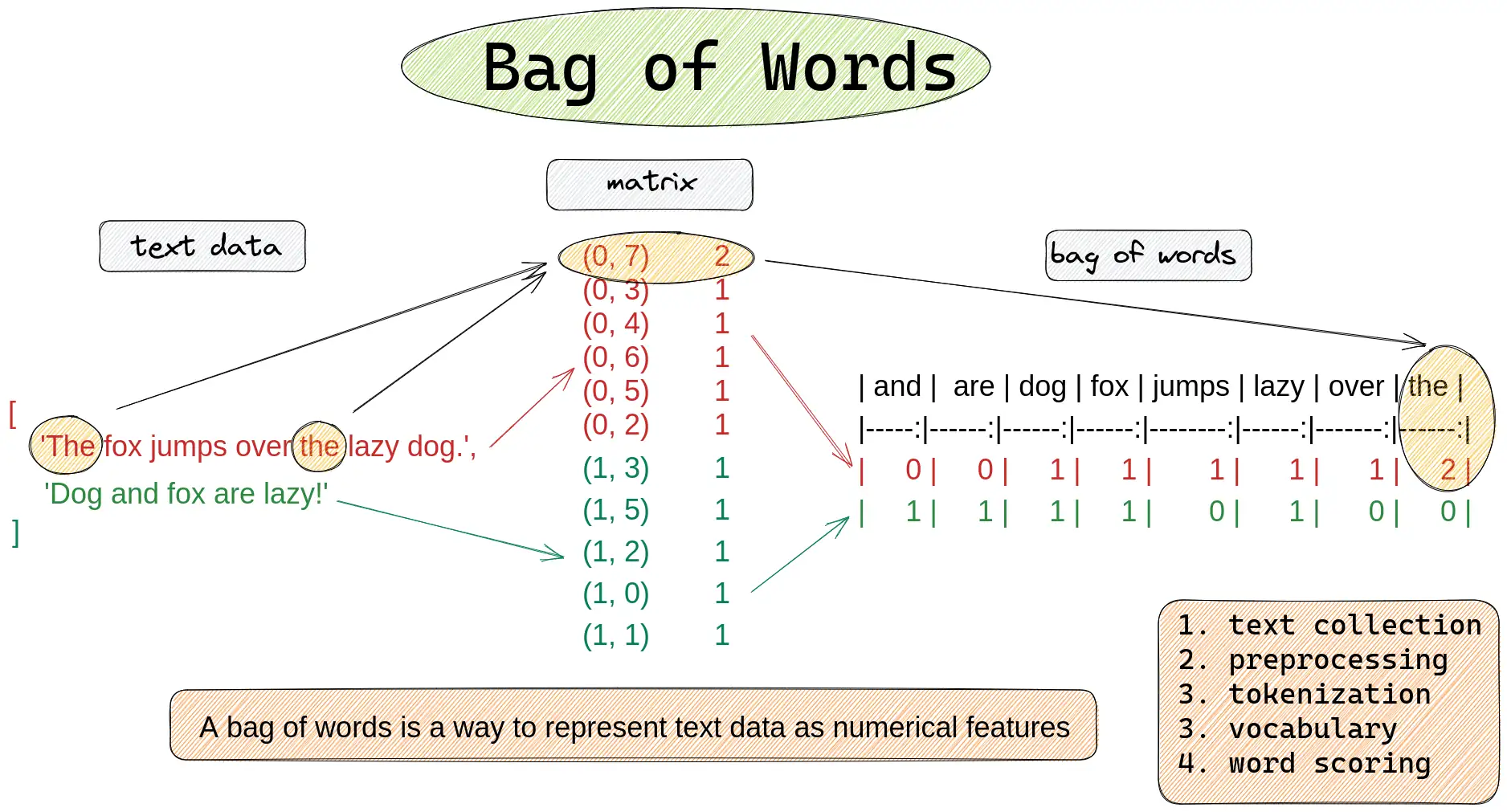
Let's see this in action and learn how to implement it using Python's scikit-learn library.
Text Representation | NLP Lecture 4 | Bag of Words | Tf-Idf | N-grams, Bi-grams and Uni-grams
This next segment from the same CampusX video provides a detailed walkthrough of the Bag-of-Words model. It covers the intuition, the implementation using CountVectorizer, and a crucial discussion of its advantages and disadvantages.
Watch from 33:17 to 57:36. As you watch, make sure you understand: How the vocabulary is built and how each document is converted into a vector of word counts. The intuition that documents with similar word counts are considered similar. How to use sklearn.feature_extraction.text.CountVectorizer to create BoW vectors automatically. The key limitations of BoW: sparsity, the out-of-vocabulary problem, and the complete loss of word order and context.
As the video discussed, one of the biggest drawbacks of BoW is that it discards word order. The sentences "man bites dog" and "dog bites man" have identical BoW representations but completely different meanings. A simple extension called N-grams can partially address this. An N-gram is a contiguous sequence of N items from a given sample of text.
- Unigrams (N=1): Single words (this is standard BoW).
- Bigrams (N=2): Pairs of adjacent words (e.g., "man bites", "bites dog").
- Trigrams (N=3): Triplets of adjacent words.
By building a vocabulary of N-grams instead of just unigrams, we can capture some local word order and context. CountVectorizer can easily be configured to use N-grams, as explained in the video from 57:36 to 01:16:24. While watching this is optional, it's a valuable technique to be aware of.
3. Method 2: TF-IDF (Term Frequency-Inverse Document Frequency)
The BoW model has another major flaw: it treats all words equally. A word like "the" might appear many times, giving it a high count, but it doesn't tell us much about the document's topic. Conversely, a word like "eigenvector" might appear only once, but it's a very strong indicator of the document's content.
We need a way to give more weight to words that are more informative. This is exactly what TF-IDF does.
TF-IDF calculates a score for each word in each document based on two factors:
- Term Frequency (TF): How often a word appears in a specific document. This is a measure of local importance.
- Inverse Document Frequency (IDF): How rare a word is across the entire corpus. This is a measure of global importance.
The final TF-IDF score is the product of these two: TF-IDF = TF * IDF.
This score is high for words that are frequent in a specific document but rare in the overall corpus, effectively highlighting the most characteristic words of that document.

Let's dive into the theory and a worked example to solidify these concepts.
TF-IDF and Bag of Words: Complete Guide
The article "TF-IDF and Bag of Words: Complete Guide to Text Representation & Information Retrieval" by Michael Brenndoerfer provides a clear, step-by-step breakdown of TF, IDF, and their combination.
Please read the following sections: 'Term Frequency (TF)': Understand the different ways to calculate TF (raw count vs. normalized). 'Inverse Document Frequency (IDF)': Grasp the intuition behind this formula and the role of the logarithm. 'TF-IDF: Combining Both Components': See how the two parts multiply to produce the final score. 'Worked Example': Follow this concrete example carefully. It walks through the BoW, IDF, and final TF-IDF calculations for a small corpus, which will make the concepts much clearer.
Implementing TF-IDF with scikit-learn
Just as CountVectorizer automates the BoW process, TfidfVectorizer in scikit-learn handles all the steps for TF-IDF. It tokenizes, builds the vocabulary, calculates TF and IDF, and returns a ready-to-use matrix of TF-IDF features.
The following video demonstrates how to use it and, importantly, applies it to a real-world text classification problem. This will show you how these vectors are used in practice and provides a perfect link to our next lesson.
Text Representation Using TF-IDF: NLP Tutorial For Beginners - S2 E6
Let's watch a video from the codebasics channel, "Text Representation Using TF-IDF". It starts with a great motivation for TF-IDF and then walks through a full coding example.
Watch the following segments: Motivation (00:00 - 07:20): This provides an excellent example of why BoW can be misleading and how IDF helps penalize generic words. Implementation (12:17 - 20:02): See how to use TfidfVectorizer to generate vocabulary, IDF scores, and the final TF-IDF matrix from a sample corpus. Application (20:02 - 35:09): This is the most important part. Follow along as the instructor applies TF-IDF to an e-commerce dataset to classify products. Notice how the TF-IDF vectors are fed into different machine learning models. This part also beautifully demonstrates how the preprocessing steps from our last lesson can improve model performance!
Conclusion
Great work! You have now mastered two fundamental and widely-used methods for turning text into numerical data that machine learning models can process. This skill is the bedrock of many NLP tasks.
Key Takeaways:
- Machine learning models require numerical input, so text must be converted into feature vectors.
- Bag-of-Words (BoW) represents documents as vectors of word counts. It's simple and fast but ignores word order and treats all words equally.
- TF-IDF improves upon BoW by weighting words. It assigns higher scores to words that are frequent in a document but rare across all documents, thus identifying the most characteristic terms.
- Both methods result in a document-term matrix, where rows are documents and columns are words from the vocabulary.
- Libraries like
scikit-learnprovide powerful and efficient tools (CountVectorizer,TfidfVectorizer) to implement these techniques in just a few lines of code.
Preview of the Next Lesson:
In the last video, you saw a preview of what's to come. We created TF-IDF vectors and immediately used them to train classification models. In the next lesson, you will learn to do this yourself, as we will focus on how to train text classification models using traditional ML techniques. You'll take the vectors we learned to create today and build models to perform tasks like sentiment analysis or topic classification.