Hello! Welcome to the third lesson in our Natural Language Processing module.
In our last two lessons, you learned how to preprocess raw text and then convert it into numerical feature vectors using Bag-of-Words and TF-IDF. You now have the skills to turn a collection of documents into a structured, numerical format that machine learning algorithms can understand.
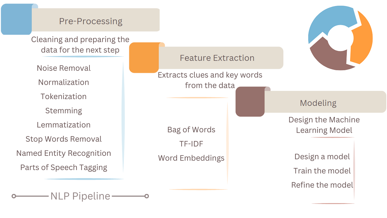
Today, we'll complete the pipeline. Your learning outcome is to train text classification models using traditional ML techniques. We'll take the TF-IDF vectors we created and use them to train and evaluate models that can automatically categorize text. This is a foundational skill for building applications like spam detectors, sentiment analyzers, and topic labelers.
1. The Core Idea: Naive Bayes for Text
Let's start with a classic and surprisingly effective algorithm for text classification: Naive Bayes. It's a probabilistic classifier based on Bayes' Theorem. For text, the core idea is:
What is the probability that a document belongs to a certain category, given the words it contains?
The "naive" part comes from its simplifying assumption that the words in a document are independent of each other. While we know this isn't true (word order and grammar matter!), the model often performs remarkably well and serves as a fantastic baseline.
To understand the mechanics of how Naive Bayes calculates these probabilities, let's watch an excellent explanation from StatQuest.
Naive Bayes, Clearly Explained!!!
The video "Naive Bayes, Clearly Explained!!!" by StatQuest with Josh Starmer provides one of the best intuitive explanations of this algorithm. We'll focus on the parts that explain the core logic and a common problem you'll encounter.
Please watch the following segments: The Main Idea (00:00 - 07:21): Focus on how the model calculates the probability of a message being 'normal' vs. 'spam' based on the probabilities of the words it contains. Pay close attention to the concepts of prior probability and how the final 'score' is calculated. The Zero-Frequency Problem (08:50 - 12:35): This part is crucial. It explains what happens when a word in a new document was never seen in a particular category during training, and how Laplace (or Additive) smoothing solves this problem.
As you saw, Naive Bayes uses word frequencies to make probabilistic guesses. The math is straightforward, making the model fast to train and easy to interpret.
2. Building a Text Classification Pipeline
Now, let's translate this theory into a practical workflow using scikit-learn. A typical text classification project involves multiple steps:
- Load the text data and labels.
- Split the data into training and testing sets.
- Vectorize the text data (e.g., using
TfidfVectorizer). - Train a classifier (e.g.,
MultinomialNB). - Evaluate the classifier on the test set.
Manually running these steps can be cumbersome, especially when you need to apply the exact same vectorization to your test data as your training data. scikit-learn provides a Pipeline object to chain these steps together into a single, cohesive unit. This is not only convenient but also prevents common errors, like accidentally re-fitting your vectorizer on the test data.
Working With Text Data — scikit-learn documentation
The official scikit-learn documentation has a fantastic tutorial on text analytics. Let's read the section that introduces the concept of a Pipeline.
Please read the section titled 'Building a pipeline'. It's short but very important. Notice how it combines the CountVectorizer, TfidfTransformer, and a classifier into one object that can be treated as a single model.
3. A Complete Code Example: Naive Bayes vs. SVM
With the concepts of Naive Bayes and Pipelines in hand, let's walk through a complete implementation. We'll use the 20 Newsgroups dataset, a classic benchmark for text classification.
We will also introduce another powerful "traditional" model: the Support Vector Machine (SVM). While Naive Bayes works with probabilities, SVM works by finding the optimal boundary (or "hyperplane") that best separates the different categories in a high-dimensional space. For many text classification tasks, SVMs are considered one of the top-performing models.
The following resource provides a clear Python implementation for classifying text using both Naive Bayes and SVM, allowing us to compare their performance directly.
Naive Bayes vs. SVM for Text Classification - GeeksforGeeks
The article "Naive Bayes vs. SVM for Text Classification" from GeeksforGeeks provides a concise comparison and a full code-along example.
Please read and follow the code in the section titled 'Naive Bayes and SVM: Python Implementation'. It walks you through every step: Loading the Dataset: Fetching the 20 Newsgroups data. Feature Extraction: Applying TfidfVectorizer to convert text to numerical features. Training Classifiers: Training both a MultinomialNB model and an SVC (Support Vector Classifier) model. Model Evaluation: Using classification_report to see how well each model performed. Since you are comfortable with Python, feel free to run this code yourself in a notebook to see it in action.
4. Choosing the Right Model
After running the code, you'll notice that SVM likely achieved a higher accuracy than Naive Bayes. This is common, but doesn't mean SVM is always better. The choice of model depends on several factors, including the dataset size, dimensionality, and the need for interpretability.
Let's quickly review the strengths and weaknesses of each model to build your intuition.
Naive Bayes vs. SVM for Text Classification - GeeksforGeeks
Let's return to the GeeksforGeeks article to understand the trade-offs between Naive Bayes and SVM.
Read the following sections: 'Naive Bayes Classifier (NB)': A quick summary of its probabilistic nature. 'Support Vector Machines (SVM)': An overview of its geometric approach (finding the best boundary). Comparison Table: Pay close attention to this table. It compares the models on criteria like efficiency, performance, scalability, and interpretability.
As a general rule of thumb for text classification:
- Naive Bayes is a great starting point. It's fast, works well with limited data, and is easy to interpret.
- SVM often provides higher accuracy, especially on complex problems, but can be slower to train on very large datasets.
In the codebasics video from our last lesson (from 20:02 onwards), you also saw an example where Random Forest outperformed Naive Bayes on an e-commerce dataset. This highlights that there's no single "best" model; experimentation is key. The pipeline you've learned to build today makes swapping out different classifiers for experimentation incredibly easy.
Conclusion
Congratulations! You have now built and evaluated your first text classification models. You've connected all the dots from raw text to a final, predictive model.
Key Takeaways:
- Text classification involves training a model on vectorized text data (like TF-IDF) to predict a category label.
- Naive Bayes is a fast, probabilistic classifier that works well as a baseline, assuming feature independence.
- Support Vector Machines (SVMs) are powerful classifiers that often yield high accuracy by finding an optimal decision boundary between classes.
scikit-learnPipelines are an essential tool for streamlining the vectorization-and-classification workflow, preventing errors and simplifying experimentation.- Model performance is evaluated using metrics like precision, recall, and F1-score, which can be easily generated with a
classification_report.
Preview of the Next Lesson:
The "traditional" models we used today are powerful, but they have a fundamental limitation: they don't understand the meaning or semantic context of words. For them, "king" and "queen" are as different as "king" and "cabbage". In the next lesson, we will begin to address this by exploring word embeddings, a technique that represents words as dense vectors in a way that captures their semantic relationships. This will be our first major step into the world of deep learning for NLP.