Hello! Welcome to the next lesson in our journey through data analysis and visualization.
In our last lesson, you mastered how to group and aggregate data using groupby and pivot_table. These are powerful tools for summarizing vast amounts of information into meaningful tables. But numbers in a table can only tell you so much. The fastest way to spot trends, relationships, and outliers is to turn those numbers into pictures.
This lesson directly follows from that, focusing on the learning outcome: Create static visualizations (line, bar, histogram, scatter) with Matplotlib. We will explore Matplotlib, the foundational plotting library in Python, to create the most common types of charts used in data analysis. This skill is a cornerstone of exploratory data analysis (EDA) and communicating your findings.
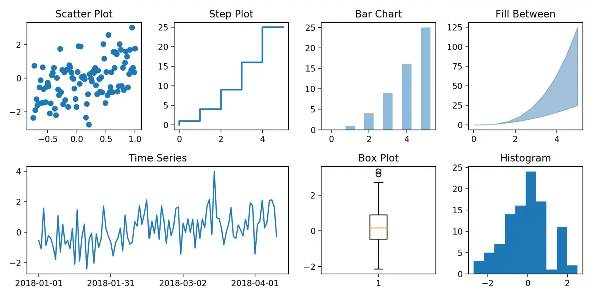
Here are some of the plots we'll be learning to create today:
The Anatomy of a Matplotlib Plot
Before we start plotting, it's essential to understand the basic structure of a Matplotlib visualization. Think of it like a painter's canvas. There are two core components:
- The
Figure: This is the entire window or page that everything is drawn on. It's the top-level container for all the plot elements. - The
Axes: This is the actual plot or chart itself, where you draw your data. A singleFigurecan contain one or moreAxes(subplots).
We will primarily use Matplotlib's Object-Oriented (OO) API. This approach involves creating explicit Figure and Axes objects and then calling methods on them. It gives you far more control and is the recommended practice for any plot that's more than a single line.
The typical setup looks like this:fig, ax = plt.subplots()
Let's start with a reading to solidify these concepts and see the recommended workflow.
Beginner's Guide To Matplotlib (With Code Examples)
The 'Beginner's Guide To Matplotlib' provides an excellent explanation of the core components of a plot and the standard workflow you'll be using.
Please read the following sections: 'Two ways of creating plots': This introduces the simple pyplot interface and the more powerful Object-Oriented (OO) API. Focus on the OO approach. 'Anatomy of a Matplotlib Figure': This clarifies the distinction between Figure, Axes, and Axis. 'An example Matplotlib workflow': This lays out the 6-step process we will follow. Internalize these steps, as they provide a reliable structure for creating any plot.
Now that you understand the structure, let's start creating some plots! We will use a comprehensive video tutorial to guide us through the practical steps for each chart type.
Creating Common Plot Types
We'll now go through the four fundamental static plot types. For each one, we'll discuss its purpose and then see how to create it using Matplotlib.
Learn Matplotlib in 30 Minutes - Python Matplotlib Tutorial
The video 'Learn Matplotlib in 30 Minutes' is a concise and practical guide. We'll use it to learn the syntax for our core plot types. Make sure you have your coding environment ready to follow along.
First, watch the introductory part from the beginning to 06:08 to get set up. The video covers: Installation and Setup (00:00 - 04:56): How to install Matplotlib and set up a Jupyter Notebook. Matplotlib Architecture (04:56 - 06:08): A quick recap of the Figure/Axes concepts we just read about.
1. Line Plot (ax.plot())
A line plot is ideal for visualizing data that changes over a continuous interval, most commonly time. It's great for showing trends.
Let's see how to create one.
Learn Matplotlib in 30 Minutes - Python Matplotlib Tutorial
Let's watch the section on creating basic and customized line plots.
Watch from 06:08 to 11:25. Pay attention to: How to create a simple line plot using plt.plot() (the pyplot interface). How to plot multiple lines on the same axes. How to customize the plot with figure size, labels, titles, and a grid. How to add a legend when you have multiple lines.
Code Summary (using the OO API):
import matplotlib.pyplot as plt
import numpy as np


# 1. Prepare Data
x = np.linspace(0, 10, 100) # 100 points from 0 to 10
y1 = np.sin(x)
y2 = np.cos(x)


# 2. Setup Plot
fig, ax = plt.subplots(figsize=(8, 5)) # Create a Figure and an Axes


# 3. Plot Data
ax.plot(x, y1, label='Sine')
ax.plot(x, y2, label='Cosine')


# 4. Customize Plot
ax.set_title('Sine and Cosine Waves')
ax.set_xlabel('X-axis')
ax.set_ylabel('Y-axis')
ax.grid(True, linestyle='--', alpha=0.6)
ax.legend()


# 5. Show Plot
plt.show()
2. Scatter Plot (ax.scatter())
A scatter plot is used to display values for two different numeric variables. It's the best way to visualize the relationship between them and spot correlations or clusters.
Learn Matplotlib in 30 Minutes - Python Matplotlib Tutorial
Now, let's learn how to create scatter plots.
Watch from 12:51 to 15:32. Notice: The switch from plot() to scatter(). How to control transparency with the alpha parameter, which is useful when points overlap. How to customize the color and size of each individual point.
Code Summary:
# 1. Prepare Data
np.random.seed(42) # for reproducible results
x = np.random.rand(50) * 10
y = x + np.random.randn(50) * 2 # y is related to x with some noise


# 2. Setup Plot
fig, ax = plt.subplots(figsize=(8, 5))


# 3. Plot Data
ax.scatter(x, y, alpha=0.7)


# 4. Customize Plot
ax.set_title('Relationship between X and Y')
ax.set_xlabel('X Value')
ax.set_ylabel('Y Value')
ax.grid(True, linestyle='--', alpha=0.6)


# 5. Show Plot
plt.show()
3. Bar Chart (ax.bar())
A bar chart is perfect for comparing quantities across different categories. This is where you can directly visualize the output of a groupby operation you learned in the previous lesson.
Learn Matplotlib in 30 Minutes - Python Matplotlib Tutorial
Next up are bar charts, a staple of data visualization.
Watch from 15:32 to 19:23. This section covers: Creating a basic vertical bar chart with bar(). Creating a horizontal bar chart with barh(). A more advanced example of a grouped bar chart for comparing sub-categories. This is a very useful technique.
Code Summary (Visualizing a groupby result):
import pandas as pd


# 1. Prepare Data (Imagine this comes from a DataFrame df)
# For example: category_summary = df.groupby('Category')['Value'].sum().reset_index()
data = {'Category': ['A', 'B', 'C', 'D'],
        'Value': [23, 45, 17, 30]}
category_summary = pd.DataFrame(data)


# 2. Setup Plot
fig, ax = plt.subplots(figsize=(8, 5))


# 3. Plot Data
ax.bar(category_summary['Category'], category_summary['Value'], color='skyblue', edgecolor='black')


# 4. Customize Plot
ax.set_title('Values per Category')
ax.set_xlabel('Category')
ax.set_ylabel('Total Value')


# 5. Show Plot
plt.show()
4. Histogram (ax.hist())
While a bar chart compares categories, a histogram shows the distribution of a single numerical variable. It groups numbers into ranges (bins) and the height of the bar shows the frequency of data in that range. It's essential for understanding the spread and skewness of your data.
Learn Matplotlib in 30 Minutes - Python Matplotlib Tutorial
Finally, let's look at histograms to understand data distributions.
Watch from 19:23 to 20:40. Focus on: The use of hist(). The bins parameter, which controls how many groups the data is divided into. How to overlay multiple histograms with transparency.
Code Summary:
# 1. Prepare Data
data = np.random.randn(1000) # 1000 data points from a standard normal distribution


# 2. Setup Plot
fig, ax = plt.subplots(figsize=(8, 5))


# 3. Plot Data
ax.hist(data, bins=30, color='lightgreen', edgecolor='black')


# 4. Customize Plot
ax.set_title('Distribution of a Numerical Variable')
ax.set_xlabel('Value')
ax.set_ylabel('Frequency')
ax.grid(True, linestyle='--', alpha=0.4)


# 5. Show Plot
plt.show()
Plotting Directly from Pandas
As a quick and convenient shortcut, pandas DataFrames have a built-in .plot() method that uses Matplotlib behind the scenes. This can be very fast for quick explorations.
The "Beginner's Guide To Matplotlib" article provides clear examples of this.
Beginner's Guide To Matplotlib (With Code Examples)
Let's see how you can generate these same plots directly from a pandas DataFrame, which is a very common workflow.
Read the section 'Plotting data directly with pandas'. Notice how you can call .plot(kind='...') on a DataFrame or Series. The kind parameter can be 'line', 'scatter', 'bar', 'hist', etc.
While convenient, remember that for fine-grained control and creating complex figures, the fig, ax = plt.subplots() method is superior.
Conclusion
Great job! You have now learned how to create the four most essential static plots for data analysis. Visualizing data is not just about making pretty pictures; it's a critical part of the analysis process that allows you to intuitively grasp complex data and effectively communicate your findings.
Key Takeaways:
- Matplotlib plots are built on a
Figure(the canvas) and one or moreAxes(the individual plots). - The Object-Oriented API (
fig, ax = plt.subplots()) provides the most power and flexibility. - Line plots (
ax.plot()) are for showing trends over a continuous range, like time. - Scatter plots (
ax.scatter()) are for visualizing the relationship between two numeric variables. - Bar charts (
ax.bar()) are for comparing quantities across discrete categories. - Histograms (
ax.hist()) are for understanding the distribution (frequency) of a single numeric variable. - Always label your plots with titles and axis labels (
ax.set_title(),ax.set_xlabel(),ax.set_ylabel()) to provide context.
In the next lesson, we will move from static to dynamic. You'll learn how to create interactive visualizations using Plotly Express. While Matplotlib is excellent for reports and publications, Plotly will allow you to build charts where users can hover for details, zoom in on areas of interest, and filter data on the fly, making for a much richer exploratory experience.