Chain Rule for Gradients in Computational Graphs

1. The Core Idea: Composing Rates of Change

Imagine a system of interconnected gears. If you know how fast the first gear turns the second, and how fast the second turns the third, you can figure out how fast the first gear turns the third by simply multiplying those rates. This is the essence of the chain rule.

To formalize this, let's start with a brief reading.

As the article states, if you have a composite function like $y=f(g(x))$, you can think of it as a chain: $x$ affects $g$, which in turn affects $f$. To find how a change in $x$ affects $y$, we multiply the derivatives of each link in the chain.

If we let $u=g(x)$, then $y=f(u)$. The chain rule is:

This simple multiplication is the key. But for a neural network with millions of parameters, the "chain" is incredibly complex. We need a way to organize this calculation.

2. Computational Graphs: Visualizing the Math

Since you have a background in programming, you're used to breaking down complex logic into smaller, manageable functions. We can do the same for mathematics using computational graphs. A computational graph represents a function as a directed graph where nodes are operations (e.g., +, *, sin) and edges represent the data flowing between them.

Why bother with this? For a complex model, deriving the full gradient expression on paper is not only tedious and error-prone but also not modular. If you change one part of your model (like the activation function), you'd have to re-derive everything. Computational graphs solve this.

As the video shows, even moderately complex neural networks produce computational graphs that are far too large to reason about manually. This is why frameworks like PyTorch and TensorFlow exist—they build this graph for you automatically. Your job is to understand the process they are executing.

This process involves two steps:

1. Forward Pass: We start with the inputs and flow through the graph from left to right, computing the value at each node until we get the final output.
2. Backward Pass: We start from the final output and flow backward from right to left, applying the chain rule at each node to compute the gradients. This backward pass is called backpropagation.

3. Backpropagation: The Chain Rule on a Graph

Let's make the backward pass more concrete. To compute the gradient at any node, we need two things:

1. The local gradient: The derivative of that node's operation with respect to its immediate inputs. (e.g., for a node c = a + b, the local gradients are $\frac{\partial c}{\partial a}=1$ and $\frac{\partial c}{\partial b}=1$).
2. The upstream gradient: The gradient of the final output with respect to the node we're at. This is passed to us from the nodes further down the chain (to the right).

The chain rule tells us that the downstream gradient (the gradient we want to pass back to the previous node) is simply:
downstream_gradient = upstream_gradient * local_gradient

Let's watch this in action.

This backward flow is incredibly efficient because it reuses computations. Once we have the gradient of the loss with respect to a layer's output, we can use it to compute the gradients for that layer's weights and pass it backward to the previous layer.

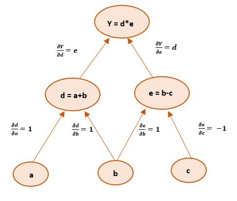
4. The Multi-Path Case: Summing Gradients

The image above hints at an important detail: what if an input variable affects the output through multiple paths?

For example, in the function f(a, b) = (a + b) * a, the variable a is used in two places. A change in a affects f through both the addition and the multiplication.

The multivariable chain rule states that in this case, we must compute the gradient along each path independently and then sum them up.

This "sum over paths" rule is the final piece of the backpropagation puzzle. It ensures we account for the total influence of a variable on the final output. The article also extends this concept to a simple neural network, showing exactly how the gradients for weights and biases are calculated. If you're curious, you can explore the rest of that article (LINK, sections 3 and 4), which shows a full numerical example and its PyTorch equivalent.

A quick note on vector and matrix operations: while our examples use scalars, real neural networks operate on tensors (vectors, matrices). The principle remains identical, but the local_gradient becomes a Jacobian matrix, and the multiplication becomes a matrix-vector product. Deep learning frameworks handle these complex operations implicitly, but they are all just executing the chain rule you've learned today.

Conclusion

You've just learned the core algorithm that enables deep learning. While it might seem complex at first, it's built from simple, repeatable steps.

Key Takeaways:

• The Chain Rule allows us to compute the derivative of a composite function by multiplying the derivatives of its constituent parts: $\frac{dy}{dx}=\frac{dy}{du}\cdot \frac{du}{dx}$.
• Computational Graphs provide a powerful way to visualize complex functions and modularize the process of differentiation.
• Backpropagation is the algorithm for efficiently computing gradients on a computational graph. It consists of:
  1. A forward pass to compute the output value.
  2. A backward pass that applies the chain rule from right to left, calculating downstream_gradient = upstream_gradient * local_gradient at each node.
• If a variable contributes to the output via multiple paths, its total gradient is the sum of the gradients from each path.

We have now concluded the calculus segment of this module. You understand how to measure rates of change (derivatives) and how to propagate them through complex functions (the chain rule).

In our next lesson, we will pivot to the second major pillar of mathematics for machine learning: Probability and Statistics. We will begin by learning how to calculate and interpret fundamental descriptive statistics like mean, variance, standard deviation, and correlation coefficients. These tools are essential for understanding and summarizing your data before you ever begin training a model.