Derivatives and Rates of Change

1. The Intuition: What is an "Instantaneous" Rate of Change?

We often talk about rates of change in everyday life—the speed of a car, the growth of a company's revenue. These are usually calculated over a period of time. But what if we want to know the rate of change at a single instant? This question presents a fascinating paradox. Change requires two points in time to measure, but an instant is just one point.

Calculus provides an elegant solution to this paradox. Let's build our intuition with a video from 3Blue1Brown, which is renowned for its excellent visual explanations.

As the video masterfully explains, the derivative is not calculated with a time interval of zero. Instead, it's the limit that the rate of change approaches as the interval dt (or more generally, Δx) shrinks towards zero.

Visually, this corresponds to finding the slope of the line tangent to the function's graph at a specific point.

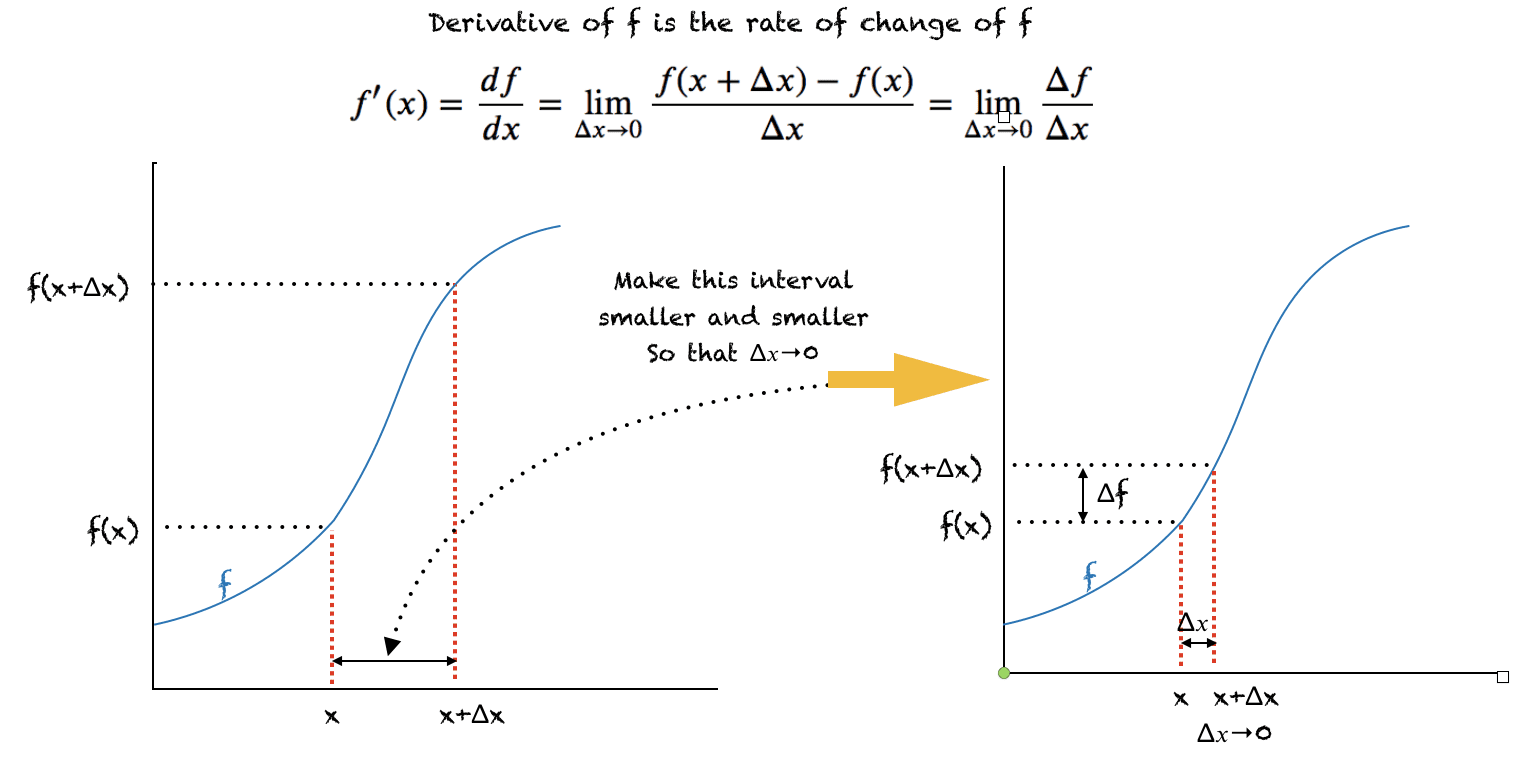
So, a derivative answers the question: "How much does my function's output change for a tiny nudge in its input?" It represents the instantaneous rate of change.

2. Calculating Derivatives: From Limits to Rules

While the limit definition is the theoretical foundation, calculating it every time would be tedious. Fortunately, mathematicians have derived simple rules for finding derivatives. For polynomial functions, the most important one is the power rule.

The Power Rule: For any function of the form $f(x)=x^n$, its derivative is $f^{\prime }(x)=n{x}^{n-1}$.

For example:

• If $f(x)=x^2$, its derivative is $f^{\prime }(x)=2x^{2-1}=2x$.
• If $f(x)=x^3$, its derivative is $f^{\prime }(x)=3x^{3-1}=3x^2$.
• If $f(x)=7x^3$, we keep the constant and apply the rule: $f^{\prime }(x)=7\cdot (3x^2)=21x^2$.

The following video provides a practical guide to applying this rule and introduces the next key concept for our lesson.

You can even write a simple Python function to approximate a derivative numerically, which directly implements the "rise-over-run" idea from the 3Blue1Brown video.

3. Partial Derivatives: Handling Multiple Inputs

Machine learning models rarely have just one input. A model predicting house prices might depend on square footage, number of bedrooms, age of the house, and so on. A loss function depends on millions of model weights. How do we find the rate of change then?

We use partial derivatives. A partial derivative measures the rate of change with respect to one variable, while treating all other variables as if they were constants.

The key insight is simple: to find the partial derivative of $f(x,y)$ with respect to $x$, you just pretend $y$ is a number (like 5 or $\pi$) and apply the normal differentiation rules.

Let's look at an example: $f(x,y)=x^2{y}^3$.

• Partial derivative with respect to x (treating $y^3$ as a constant):
  $\frac{\partial f}{\partial x}=y^3\cdot (2x)=2x{y}^3$
• Partial derivative with respect to y (treating $x^2$ as a constant):
  $\frac{\partial f}{\partial y}=x^2\cdot (3y^2)=3x^2{y}^2$

The symbol $\partial$ (called "del") is used to signify a partial derivative.

Let's return to the codebasics video to see this explained in the context of a practical example.

The geometric intuition for partial derivatives is powerful. If a function of two variables creates a 3D surface (like a landscape), taking a partial derivative is like taking a 2D "slice" through that landscape and finding the slope of the resulting curve.

For a more detailed explanation of the notation and intuition, the following reading is excellent.

4. The Gradient: A Vector of Partial Derivatives

When we have a function with multiple variables, we can compute the partial derivative for each one. If we collect all of these partial derivatives into a vector, we get the gradient, denoted by $\nabla f$.

For a function $f(x,y,z)$, the gradient is:
$\nabla f=\left[\begin{array}{c}\frac{\partial f}{\partial x}\\ \frac{\partial f}{\partial y}\\ \frac{\partial f}{\partial z}\end{array}\right]$

The gradient vector is arguably the single most important concept in modern machine learning. Why? Because it points in the direction of the steepest ascent of the function. If you want to increase a function's value as quickly as possible (e.g., maximize profit), you should move in the direction of the gradient. If you want to decrease it as quickly as possible (e.g., minimize error), you move in the opposite direction. This is the core idea behind gradient descent, the optimization algorithm that powers the training of most neural networks.

Conclusion

In this lesson, we laid the groundwork for understanding how machine learning models learn. We moved from the abstract concept of an "instantaneous rate of change" to the practical tools of derivatives and partial derivatives.

Key Takeaways:

• Derivative: The derivative of a function at a point measures its instantaneous rate of change, which is geometrically interpreted as the slope of the tangent line at that point.
• Power Rule: A simple rule for calculating derivatives of polynomial functions: the derivative of $x^n$ is $n{x}^{n-1}$.
• Partial Derivative: Measures the rate of change of a multi-variable function with respect to one variable, while holding all others constant. This is crucial for understanding the effect of individual features or weights in a model.
• Gradient: A vector that bundles together all the partial derivatives of a function. It points in the direction of the function's steepest increase.

In our next lesson, we will learn about the chain rule. While the power rule is great for simple functions, machine learning models are complex, nested functions (functions within functions). The chain rule is the key that will unlock our ability to compute gradients for these complex models, a process you will come to know as backpropagation.