Eigenvalues and Eigenvectors: Calculation and Geometric Interpretation

1. The Geometric Meaning: Special Vectors of a Transformation

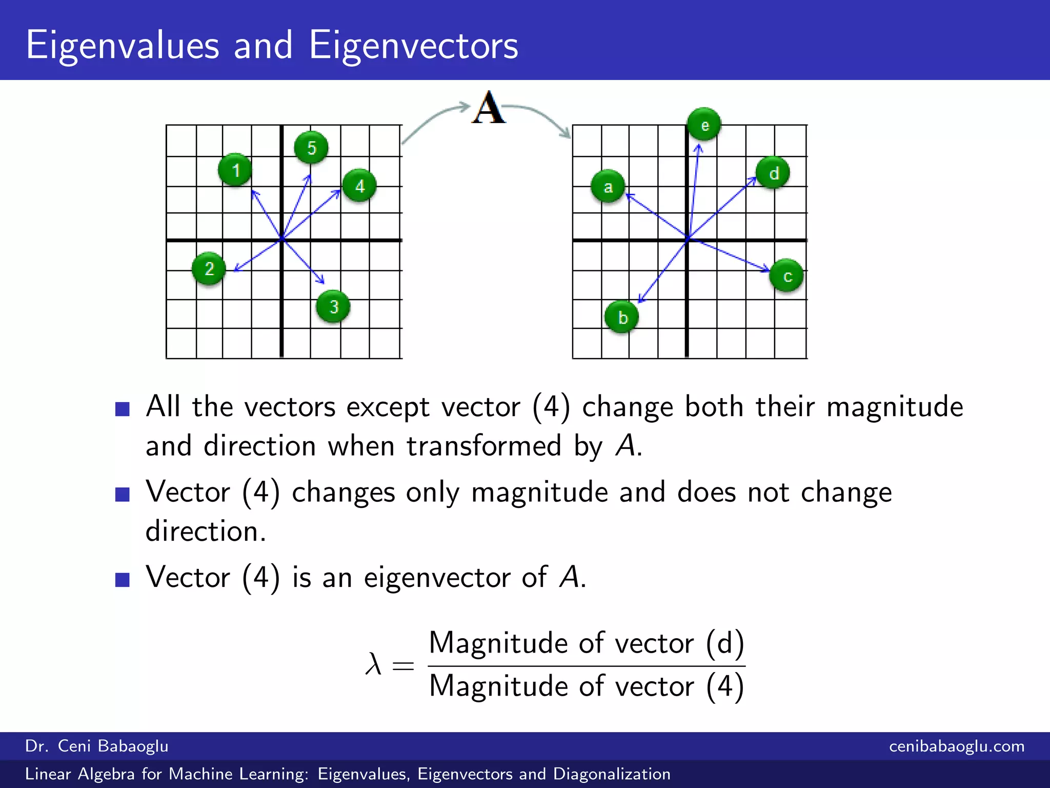
Imagine a linear transformation squishing, stretching, and rotating space. Most vectors will be knocked off their original line. However, some special vectors will simply be stretched or shrunk, perfectly maintaining their original direction. These are the eigenvectors. The factor by which they are stretched or shrunk is their corresponding eigenvalue.

To build a strong intuition for this, there's no better resource than 3Blue1Brown.

As the video explains, this concept is incredibly powerful. For a 3D rotation, the eigenvector is the axis of rotation—the one direction that remains stable. In data analysis, eigenvectors can represent the principal directions of variance in your data (a topic we'll see in Principal Component Analysis, or PCA).

2. How to Calculate Eigenvalues and Eigenvectors

Now that we have the intuition, let's dive into the calculation. The formal definition of an eigenvector $\mathbf{v}$ and its corresponding eigenvalue $\lambda$ for a matrix $\mathbf{A}$ is:

$\mathbf{Av}=\lambda \mathbf{v}$

This equation states that when the matrix $\mathbf{A}$ transforms the vector $\mathbf{v}$, the result is the same as simply scaling $\mathbf{v}$ by the scalar $\lambda$.

To solve for $\lambda$ and $\mathbf{v}$, we can't just divide by $\mathbf{v}$. We need a bit of algebra. The process involves two main steps: first finding the eigenvalues, then finding the corresponding eigenvectors.

The video below gives a very clear, step-by-step guide to this process.

Let's summarize the procedure you just saw.

Step 1: Find the Eigenvalues ($\lambda$)

1. Start with the defining equation: $\mathbf{Av}=\lambda \mathbf{v}$.
2. Rearrange it to find a vector $\mathbf{v}$ that gets sent to the zero vector.
   $\mathbf{Av}-\lambda \mathbf{v}=0$
   $\mathbf{Av}-\lambda \mathbf{Iv}=0(\text{where }\mathbf{I}\text{ is the identity matrix})$
   $(\mathbf{A}-\lambda \mathbf{I})\mathbf{v}=0$
3. This equation states that the matrix $(\mathbf{A}-\lambda \mathbf{I})$ transforms a non-zero vector $\mathbf{v}$ into the zero vector. As you saw in the 3Blue1Brown video, this can only happen if the transformation squishes space into a lower dimension—meaning the matrix is not invertible and its determinant is zero.
4. This gives us the characteristic equation, which we can solve for $\lambda$:
   $\det (\mathbf{A}-\lambda \mathbf{I})=0$
   The solutions for $\lambda$ are the eigenvalues of matrix $\mathbf{A}$. For an $n\times n$ matrix, this will be a polynomial of degree $n$, giving up to $n$ distinct eigenvalues.

Step 2: Find the Eigenvectors ($\mathbf{v}$)

1. For each eigenvalue $\lambda$ you found, plug it back into the equation:
   $(\mathbf{A}-\lambda \mathbf{I})\mathbf{v}=0$
2. This gives you a system of linear equations. Solve for the vector $\mathbf{v}=[x_1,x_2,\dots {]}^{\top }$.
3. The solution will not be a single unique vector, but rather a set of vectors that all lie on the same line (or in the same subspace). As Professor Dave showed, you can "choose" a simple value for one of the components (like $x_1=1$) to get a representative eigenvector. Any scalar multiple of that vector is also a valid eigenvector.

3. From Manual Calculation to Python Code

While it's crucial to understand the manual calculation, in practice, you'll always use a library like NumPy to find eigenvalues and eigenvectors.

The numpy.linalg.eig() function does all this work for you. Let's see how to use it.

Let's use the first example from the Professor Dave video and verify it with NumPy.
The matrix was:
$\mathbf{A}=\left[\begin{array}{cc}1& 1\\ 4& 1\end{array}\right]$
He calculated the eigenvalues to be ${\lambda }_1=3$ and ${\lambda }_2=-1$, with corresponding eigenvectors ${\mathbf{v}}_1=[1,2{]}^{\top }$ and ${\mathbf{v}}_2=[1,-2{]}^{\top }$.

Now, let's do it in Python:

import numpy as np




# Define the matrix A
A = np.array([[1, 1],
              [4, 1]])




# Calculate eigenvalues and eigenvectors
eigenvalues, eigenvectors = np.linalg.eig(A)

print("Eigenvalues from NumPy:")
print(eigenvalues)

print("\nEigenvectors from NumPy:")
print(eigenvectors)

You'll notice two things about the NumPy output:

1. The eigenvalues [ 3., -1.] match the manual calculation perfectly.
2. The eigenvectors look different: [[ 0.447, -0.447], [ 0.894, 0.894]].

Why the difference? numpy.linalg.eig returns normalized eigenvectors, meaning their length (L2 norm) is 1. Let's check: the eigenvector for $\lambda =3$ is approximately [0.447, 0.894]. If you divide our manually calculated vector [1, 2] by its length, $\sqrt{1^2+2^2}=\sqrt{5}\approx 2.236$, you get [1/2.236, 2/2.236], which is [0.447, 0.894]. They are the same vector, just scaled differently. Remember, any non-zero scalar multiple of an eigenvector is still an eigenvector.

4. Why This Matters for AI: A Glimpse into Deep Learning

Eigenvalues are not just a mathematical curiosity. They can tell you about the stability of a system. In a neural network, each layer is essentially a matrix multiplication followed by a non-linear activation. If we simplify and imagine a deep network as just repeated matrix multiplications (${\mathbf{A}}^N{\mathbf{v}}_{in}$), the behavior is dominated by the largest eigenvalue of $\mathbf{A}$.

• If the largest eigenvalue's magnitude is > 1, the output vector will grow exponentially with each layer, leading to exploding gradients.
• If the largest eigenvalue's magnitude is < 1, the output vector will shrink to zero, leading to vanishing gradients.

Proper initialization of network weights is designed to keep the largest eigenvalue around 1, ensuring signals can propagate through the network without exploding or vanishing.

Conclusion

In this lesson, we demystified the concepts of eigenvalues and eigenvectors. They are the intrinsic directions and scaling factors of a linear transformation, revealing its fundamental properties.

Key Takeaways:

• Geometric Significance: Eigenvectors are special vectors that a matrix transformation only scales, without changing their direction. The eigenvalue is that scaling factor.
• Calculation: Eigenvalues ($\lambda$) are found by solving the characteristic equation $\det (\mathbf{A}-\lambda \mathbf{I})=0$. Eigenvectors ($\mathbf{v}$) are then found by solving $(\mathbf{A}-\lambda \mathbf{I})\mathbf{v}=0$ for each eigenvalue.
• Practical Computation: In practice, you will use functions like numpy.linalg.eig() to compute them instantly.
• Relevance to AI: Eigenvalues are critical for analyzing the stability of dynamic systems, including deep neural networks, where they help us understand and prevent issues like exploding or vanishing gradients.

In our next lesson, we will shift our focus from transformations to optimization. We will learn how to calculate derivatives and partial derivatives, which measure rates of change. This will lead us directly to the concept of the gradient, the single most important tool for training machine learning models.