Hello! Welcome to your next lesson in the "Mathematics for Machine Learning" module.
In our previous lessons, we delved into the world of calculus, culminating in understanding the chain rule and its application in backpropagation—the engine that powers neural network training. We've now completed the calculus portion of this module.
Today, we pivot to the second major pillar of mathematics for machine learning: Probability and Statistics. We'll start with the fundamentals of descriptive statistics, which are essential for the first step of any data-driven project: understanding your data.
This lesson covers the learning outcome: Calculate mean, variance, standard deviation, and correlation coefficients. By the end of this lesson, you will be able to:
- Describe a dataset's central tendency using the mean.
- Quantify the spread or dispersion of data using variance and standard deviation.
- Measure the direction and strength of a linear relationship between two variables using covariance and correlation.
- Implement these calculations in Python using NumPy.
Let's begin by exploring how to summarize a dataset with a single number that represents its "center."
1. Measures of Central Tendency: The Mean
The most common way to measure the central point of a dataset is by calculating the mean, or average. It gives us a quick summary of the typical value we might expect from the data.
An important distinction in statistics is whether you are working with the entire population (all possible data points) or a sample (a subset of the population).
- The population mean, denoted by the Greek letter (mu), is the true average of the entire population.
- The sample mean, denoted by ("x-bar"), is the average of your sample. We use it to estimate the population mean.
For practical purposes in machine learning, we almost always work with samples.
The formula for the mean is straightforward: sum all the values and divide by the count of values.
While simple, the mean has one major weakness: it is highly sensitive to outliers (extremely high or low values).
Statistics Fundamentals for Machine Learning Part-1
This article from Medium provides a clear definition of the mean and a great example illustrating its sensitivity to outliers.
Read the section 'Measure of Central Tendency' and the subsection '(i) Mean'. Pay close attention to the salary example, which demonstrates how a single outlier can skew the mean.
2. Measures of Dispersion: Variance and Standard Deviation
The mean tells us about the center of our data, but it doesn't tell us anything about its spread. For instance, the datasets [0, 10, 20] and [9, 10, 11] both have a mean of 10, but their distributions are clearly very different. We need a way to measure this spread.
This is where variance and standard deviation come in.
- Variance measures the average squared difference of each data point from the mean. A larger variance means the data is more spread out.
- Standard Deviation is simply the square root of the variance. Its key advantage is that it is in the same units as the original data, making it much more interpretable.
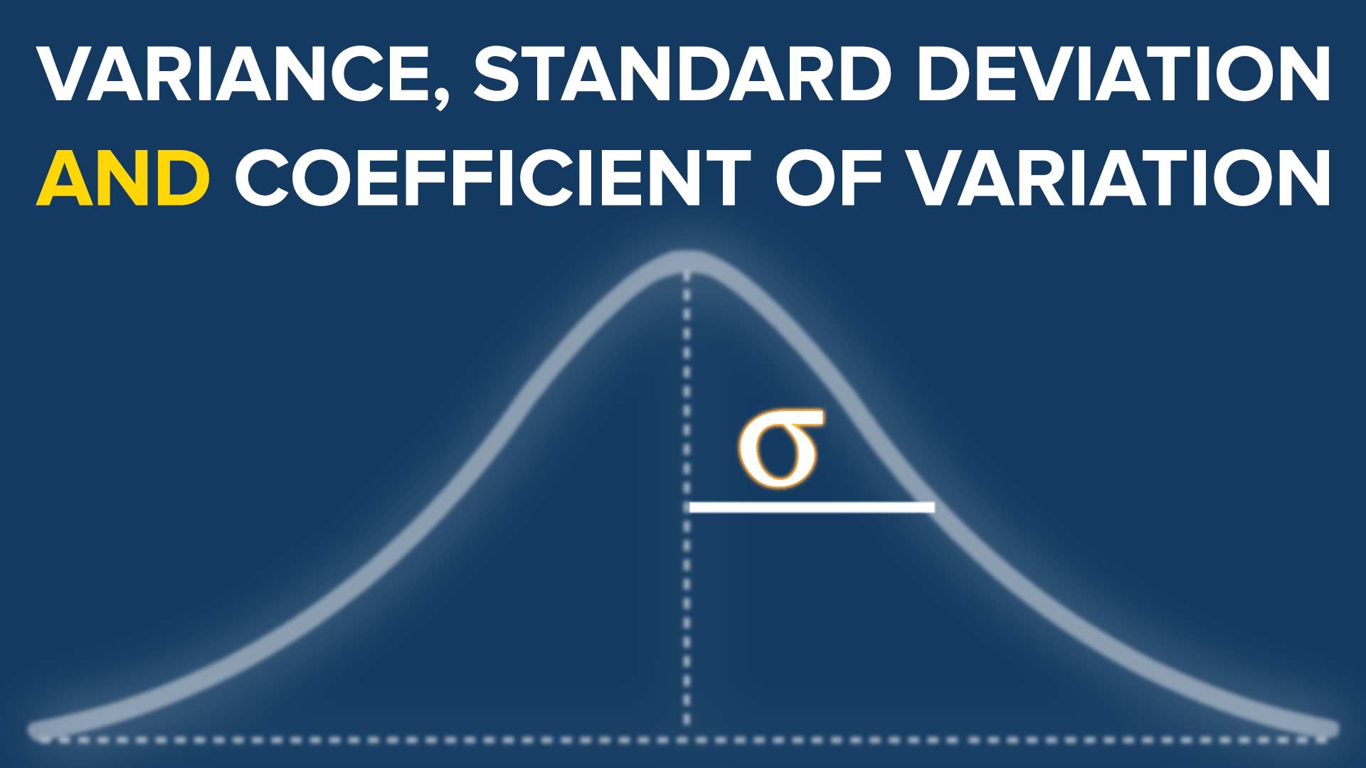
Calculating these also involves a distinction between population and sample, with a subtle but critical difference in the formula. To understand these concepts and the "why" behind the formulas, let's watch a classic StatQuest video.
Calculating the Mean, Variance and Standard Deviation, Clearly Explained!!!
This video from StatQuest with Josh Starmer offers an exceptionally clear explanation of mean, variance, and standard deviation. It beautifully clarifies the difference between population and sample formulas.
Watch from the beginning to the end (00:00 - 13:03). Pay close attention to: The conceptual difference between population and sample (02:48). Why we square the differences when calculating variance (05:20). The crucial n-1 denominator for sample variance and why it's used to get a better estimate (07:12).
To summarize the key formulas from the video:
| Measure | Population (True Value) | Sample (Estimate) |
|---|---|---|
| Variance | ||
| Std. Dev. |
The use of in the denominator for sample calculations is known as Bessel's correction. It corrects the tendency of the sample variance to be slightly smaller than the true population variance. Most statistical software, including NumPy, uses this denominator by default.
3. Measures of Relationship: Covariance and Correlation
So far, we've only described single variables. But in machine learning, we're often interested in the relationship between variables. For example, does a student's study time affect their exam score?
Covariance measures how two variables change together.
- Positive Covariance: When one variable increases, the other tends to increase.
- Negative Covariance: When one variable increases, the other tends to decrease.
- Zero Covariance: No linear relationship.
The formula for sample covariance is:
While useful for determining the direction of a relationship, the magnitude of covariance is difficult to interpret because it's dependent on the units of the variables. For example, the covariance between height (in meters) and weight (in kg) will be vastly different from the covariance between height (in cm) and weight (in grams), even for the same data.
This is solved by correlation. The Pearson correlation coefficient is a normalized version of covariance. It scales the value to be between -1 and +1, giving us a standardized measure of the strength and direction of a linear relationship.
- +1: Perfect positive linear relationship.
- -1: Perfect negative linear relationship.
- 0: No linear relationship.
This video from Normalized Nerd provides a great visual intuition for covariance and explains why we need the correlation coefficient.
Watch from 02:08 to 06:26. Focus on: The visual explanation of how points contribute to positive or negative covariance (02:08 - 04:17). How correlation normalizes covariance to give a value between -1 and 1 (05:01 - 05:59). The critical takeaway that correlation does not imply causation (05:59 - 06:26).
This last point is arguably one of the most important principles in all of statistics. Just because two variables are correlated doesn't mean one causes the other. There could be a third, unobserved variable (a "confounding variable") causing both to change.
4. Practical Implementation with NumPy
Now, let's connect these concepts to code. The NumPy library, which you've already started using, makes calculating these statistics trivial.
This tutorial from TutorialsPoint shows the NumPy functions for the statistics we've just discussed. This will bridge the gap from mathematical theory to practical Python implementation.
Read the sections 'The numpy.mean() Function', 'The numpy.std() Function', 'The numpy.var()Function', and 'Correlation Coefficient'. You can skim the examples for axis and weights for now, but focus on the basic usage of each function.
Here's a quick summary with a hands-on example. Let's imagine we have data on hours studied and exam scores.
import numpy as np


# Sample data: [hours_studied, exam_score]
hours_studied = np.array([2, 3, 5, 7, 8])
exam_scores = np.array([65, 70, 75, 85, 90])


# 1. Calculate Mean
mean_hours = np.mean(hours_studied)
mean_scores = np.mean(exam_scores)
print(f"Mean hours studied: {mean_hours:.2f}")
print(f"Mean exam score: {mean_scores:.2f}\n")


# 2. Calculate Variance and Standard Deviation
# By default, np.var and np.std use the population formula (ddof=0).
# For sample statistics, set ddof=1 (ddof stands for 'Delta Degrees of Freedom').
# This makes the denominator n-1 instead of n.
var_scores_sample = np.var(exam_scores, ddof=1)
std_scores_sample = np.std(exam_scores, ddof=1)
print(f"Sample variance of scores: {var_scores_sample:.2f}")
print(f"Sample standard deviation of scores: {std_scores_sample:.2f}\n")


# 3. Calculate Covariance and Correlation
# np.corrcoef returns a 2x2 matrix
# The value at [0, 1] is the correlation between the two variables
correlation_matrix = np.corrcoef(hours_studied, exam_scores)
correlation = correlation_matrix[0, 1]
print("Correlation Matrix:\n", correlation_matrix)
print(f"\nCorrelation between hours studied and exam scores: {correlation:.2f}")
The correlation coefficient of approximately 0.98 indicates a very strong positive linear relationship, which matches our intuition: more hours studied is associated with higher exam scores.
Conclusion
You have just learned the foundational tools for describing and summarizing data. These metrics are the first things you will calculate when you encounter a new dataset, forming the backbone of Exploratory Data Analysis (EDA).
Key Takeaways:
- Mean: Measures the central tendency of data but is sensitive to outliers.
- Variance & Standard Deviation: Measure the spread or dispersion of data. Standard deviation is more interpretable as it's in the original units.
- Sample vs. Population: When estimating from a sample, we use in the denominator for variance (Bessel's correction) to get a more accurate estimate of the population variance.
- Covariance: Measures the direction of a linear relationship between two variables.
- Correlation Coefficient: A normalized version of covariance () that measures both the strength and direction of a linear relationship.
- Correlation is not Causation: A strong correlation does not prove that one variable causes the other.
In our next lesson, we will build upon this foundation and dive deeper into the world of probability. We will formally define key concepts like sample space, events, and conditional probability, which are the building blocks for understanding more advanced machine learning models.