Convolutional Neural Networks: Building Blocks

1. Why Standard Neural Networks Fail for Images

Before we learn about CNNs, let's understand the problem they were designed to solve. Imagine feeding a simple 256x256 pixel grayscale image to the feedforward neural networks we've studied so far. You would first have to flatten the image into a single vector of $256\times 256=65,536$ pixel values.

This approach has two major flaws:

1. Computational Cost: The first hidden layer would have an enormous number of weights. If it had just 1000 neurons, you'd already be looking at over 65 million weights ($65,536\times 1000$) just for that one layer. This is computationally expensive and highly prone to overfitting.
2. Loss of Spatial Information: When you flatten an image, you throw away its structure. The network loses the information that pixels are arranged in a 2D grid, where neighboring pixels are highly related. It treats a pixel in the top-left corner the same as a pixel in the bottom-right.

To see a great illustration of these challenges, let's watch a short video.

As the video explains, the key is to stop looking at the image as one giant vector and start looking for small, local patterns or features, just like our brains do. This is the core idea behind the convolution operation.

2. The Convolution Operation: Finding Features with Filters

The convolution is the central building block of a CNN. Instead of connecting every input pixel to every neuron, a convolutional layer uses a small matrix called a filter (or kernel) to scan the image and detect specific features.

Here's how it works:

1. The filter, which is much smaller than the image (e.g., 3x3 or 5x5), is placed over a patch of the image starting at the top-left.
2. An element-wise multiplication is performed between the filter's values and the pixel values of the image patch it's covering.
3. The results of the multiplication are summed up to produce a single number.
4. This number is placed in the corresponding position of a new matrix, called a feature map or activation map.
5. The filter then slides over to the next patch of the image, and the process repeats until the entire image has been scanned.

The resulting feature map shows where the feature detected by the filter appears in the image. For example, one filter might be trained to detect vertical edges, another to detect horizontal edges, and another a specific color or texture.

Let's watch a detailed, step-by-step visualization of this process.

To solidify these concepts with more formal terminology, let's turn to a foundational text in this field.

The magic of convolution lies in parameter sharing. Instead of learning a separate weight for every pixel, we learn a single set of weights for a filter, which is then applied across the whole image. This dramatically reduces the number of parameters and makes the network translation invariant: a feature learned in one part of the image can be detected anywhere else.

3. Stride: Controlling the Filter's Movement

Stride specifies how many pixels the filter moves at each step as it slides across the input image.

• A stride of 1 means the filter moves one pixel at a time, resulting in a dense scan and a large output feature map that overlaps heavily.
• A stride of 2 means the filter jumps two pixels at each step, horizontally and vertically. This results in a smaller output feature map because the filter is applied to fewer locations.

The size of the output feature map can be precisely calculated. The formula is:

$\text{Output Size}=\frac{(W-F+2P)}{S}+1$

Where:

• $W$ is the input volume size (e.g., width or height).
• $F$ is the filter size.
• $P$ is the amount of padding (we'll cover padding in more detail later, for now assume $P=0$).
• $S$ is the stride.

Let's look at a quick resource that defines stride clearly.

Choosing a stride is a trade-off. A smaller stride preserves more spatial information but is computationally more expensive. A larger stride acts as a form of downsampling, reducing the size of the feature maps and the overall computation.

4. Pooling: Downsampling and Summarizing Features

After a convolution operation, it's common to apply a pooling layer. The primary purpose of pooling is to reduce the spatial dimensions (width and height) of the feature maps.

This has several benefits:

• It reduces the number of parameters and computational load in the network.
• It helps to control overfitting by summarizing features in a neighborhood, making the representation more robust.
• It provides a small degree of translation invariance; the exact location of a feature becomes less important, only its presence in a region matters.

The most common type of pooling is Max Pooling. It works by sliding a window (e.g., 2x2) over the feature map and, for each region, taking only the maximum value.

Let's see this in action.

Now, let's read a concise summary of the pooling layer.

Together, convolution and pooling form the core feature extraction engine of a CNN. A typical CNN architecture will stack multiple layers of Convolution -> Pooling to learn a hierarchy of features. Early layers might learn simple features like edges and colors, while deeper layers combine these to learn more complex features like eyes, faces, or wheels.

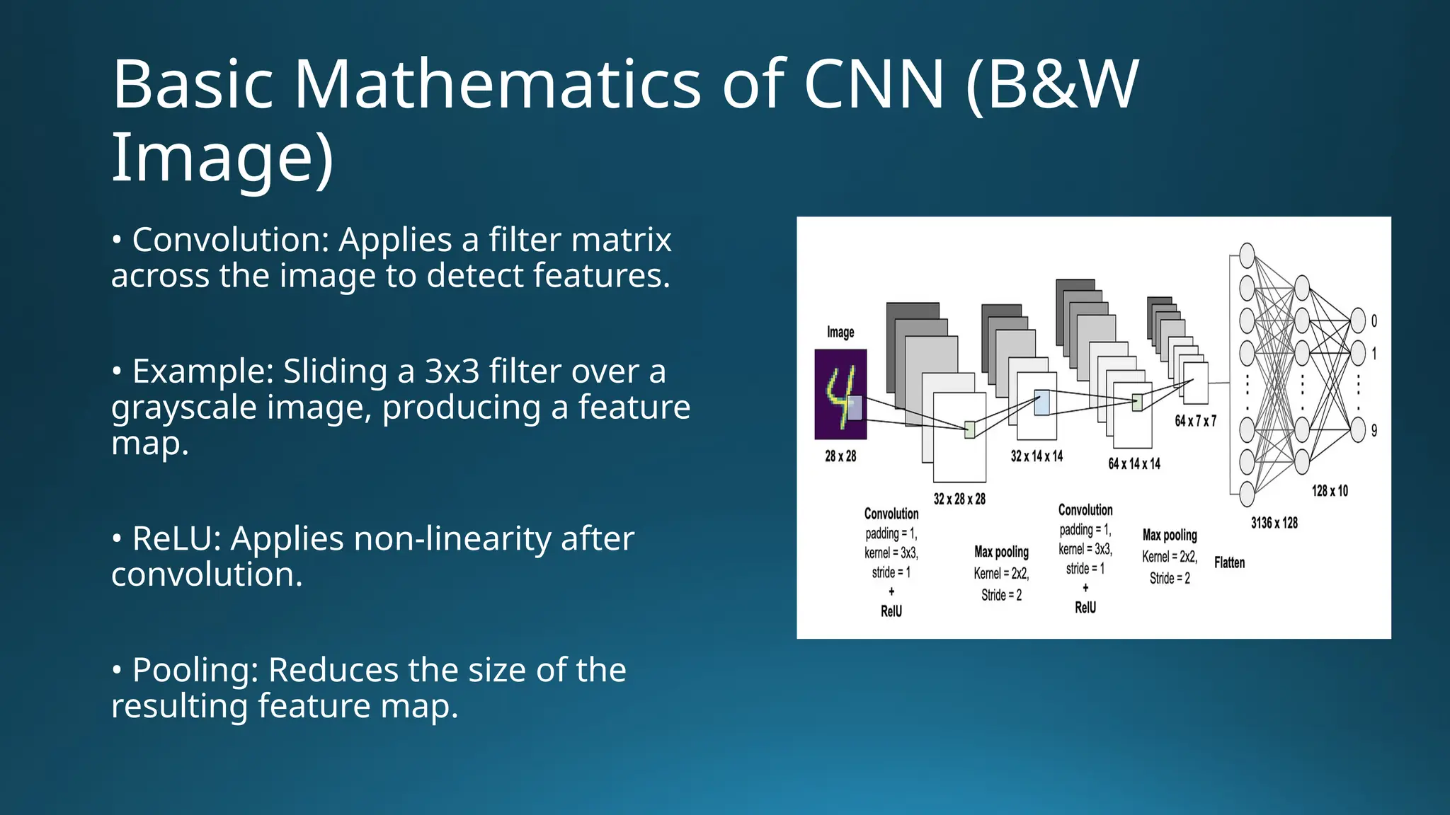
Conclusion

In this lesson, we've unpacked the fundamental mechanics of Convolutional Neural Networks. You now understand the "what" and "why" behind the operations that make CNNs so effective for image analysis.

Key Takeaways:

• Standard neural networks are ill-suited for images due to the high number of parameters and loss of spatial information.
• The convolution operation uses filters (kernels) to scan an image and create feature maps, which highlight the locations of specific patterns like edges or textures. This relies on the principle of parameter sharing.
• Stride is the step size the filter takes as it moves across the image. A larger stride reduces the output size and computation.
• The pooling layer (commonly max pooling) downsamples feature maps to reduce dimensionality, control overfitting, and provide a degree of translation invariance.

Preview of the Next Lesson:
Theory is great, but putting it into practice is better. In the next lesson, "Build and train a CNN for image classification using PyTorch," we will take these concepts and use them to build our very first CNN from scratch. You will see how to define convolutional and pooling layers in PyTorch and train a complete model to classify images.