PyTorch CNNs for Image Classification

The End-to-End Workflow

Building and training a neural network follows a standard, repeatable process. We will implement the following five steps, which you'll use in almost every deep learning project:

1. Load and normalize the data: We'll use the popular CIFAR-10 image dataset and prepare it for our network.
2. Define the CNN architecture: We'll construct the network by stacking convolutional, pooling, and fully connected layers.
3. Define a loss function and optimizer: We'll choose the appropriate tools to measure our model's error and update its weights.
4. Train the network: We'll feed the training data to the model and let it learn.
5. Test the network: We'll evaluate how well our trained model performs on unseen data.

This entire pipeline is visualized below, showing how an image flows through the layers to produce a final classification.

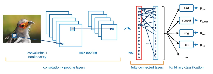
1. Loading and Preparing the Data

The first step is to get our data ready. PyTorch's torchvision library makes it incredibly simple to work with standard image datasets. We will use the CIFAR-10 dataset, which consists of 60,000 32x32 color images in 10 classes (e.g., 'plane', 'car', 'bird').

When loading the data, we also need to apply some transformations:

• transforms.ToTensor(): This converts the images from their original format (PILImage) into PyTorch tensors. It also scales the pixel values from a range of [0, 255] to [0, 1].
• transforms.Normalize(): This normalizes the tensor's values. By providing the mean and standard deviation for each of the three color channels (Red, Green, Blue), it scales the values to be in the range [-1, 1]. This helps the network train more stably and efficiently.

Finally, we'll wrap our dataset in a DataLoader, which is a utility that provides batches of data, shuffles it for each epoch, and can even use multiple subprocesses to load data in parallel.

For a clear, code-driven walkthrough of this process, please read the first section of the official PyTorch tutorial on this topic.

2. Defining the CNN Architecture in PyTorch

This is where we build our network. In PyTorch, a model is defined as a Python class that inherits from torch.nn.Module.

The architecture consists of two main parts:

1. __init__(): The constructor where we define all the layers our network will use. We'll be using nn.Conv2d for convolutional layers, nn.MaxPool2d for pooling, and nn.Linear for the final classification layers.
2. forward(): This method defines the "forward pass"—how an input tensor x flows through the layers we defined in __init__().

Let's watch a detailed video that walks through creating a CNN class, paying special attention to a common challenge: calculating the correct input size for the first fully connected (Linear) layer.

To solidify your understanding, here is the complete code for the network architecture from the official PyTorch tutorial. You can see it matches the structure described in the video.

import torch.nn as nn
import torch.nn.functional as F

class Net(nn.Module):
    def __init__(self):
        super().__init__()



        # 3 input image channels (RGB), 6 output channels, 5x5 square convolution kernel
        self.conv1 = nn.Conv2d(3, 6, 5)



        # Max pooling over a (2, 2) window
        self.pool = nn.MaxPool2d(2, 2)
        self.conv2 = nn.Conv2d(6, 16, 5)



        # an affine operation: y = Wx + b
        self.fc1 = nn.Linear(16 * 5 * 5, 120)  # <-- The result of the calculation from the video
        self.fc2 = nn.Linear(120, 84)
        self.fc3 = nn.Linear(84, 10) # 10 output classes

    def forward(self, x):



        # Apply conv1, then ReLU, then pooling
        x = self.pool(F.relu(self.conv1(x)))



        # Apply conv2, then ReLU, then pooling
        x = self.pool(F.relu(self.conv2(x)))



        # Flatten all dimensions except the batch dimension
        x = torch.flatten(x, 1) 



        # Apply linear layers with ReLU activations
        x = F.relu(self.fc1(x))
        x = F.relu(self.fc2(x))



        # Final output layer (no activation, as CrossEntropyLoss will handle it)
        x = self.fc3(x)
        return x

net = Net()
print(net)

3. Training the Network

With our data prepared and our network defined, the final steps are to set up and run the training process. This part will be very similar to what you saw in the "Deep Learning Foundations" module.

1. Define Loss Function and Optimizer: For multi-class classification, nn.CrossEntropyLoss is the standard choice. It combines a LogSoftmax layer and a Negative Log-Likelihood loss in one class. For the optimizer, torch.optim.SGD with momentum is a classic and solid choice.

2. The Training Loop: We will loop over our dataset for a specified number of epochs. In each epoch, we loop through the trainloader, which gives us batches of [inputs, labels]. For each batch, we perform the following steps:

   • Zero the gradients (optimizer.zero_grad()).
   • Perform a forward pass to get the model's predictions (outputs = net(inputs)).
   • Calculate the loss (loss = criterion(outputs, labels)).
   • Perform backpropagation to compute gradients (loss.backward()).
   • Update the model's weights (optimizer.step()).

Let's watch a video that brings all these pieces together and shows the full implementation from start to finish.

As a reference, you can find the corresponding code for defining the loss/optimizer and the training loop in sections 3 and 4 of the PyTorch tutorial we looked at earlier ([LINK](https://docs.pytorch.org/tutorials/beginner/blitz/cifar10_tutorial.html)).

4. Evaluating the Model

After training, we need to see how well our model has learned. We do this by making predictions on the test set—data the model has never seen before.

The process is straightforward:

1. Set the model to evaluation mode with net.eval(). This disables layers like Dropout that behave differently during training and inference.
2. Use a with torch.no_grad(): block. This tells PyTorch not to calculate gradients, which saves memory and computation since we are not training.
3. Loop through the testloader, pass the images through the network, and get the predicted class by finding the index of the highest output value using torch.max().
4. Compare the predicted classes to the true labels and calculate the accuracy.

This final step is covered in the last part of the PyTorch tutorial.

The accuracy you get might be around 50-60%. While not state-of-the-art, it's significantly better than the 10% accuracy of random guessing, proving that our network has successfully learned features from the images!

Conclusion

Congratulations! You have now walked through the entire process of building and training a Convolutional Neural Network in PyTorch. You've combined the theoretical concepts from the last lesson with the practical coding skills from your Python and PyTorch foundation.

Key Takeaways:

• The entire process follows a standard workflow: Data -> Model -> Loss/Optimizer -> Train -> Evaluate.
• torchvision and DataLoader are powerful tools for loading and preparing image datasets.
• A CNN model is defined as a class inheriting from nn.Module, with layers defined in __init__ and the data flow defined in forward.
• A critical step is to calculate the flattened feature size to correctly connect nn.Conv2d layers to nn.Linear layers.
• The training loop iterates through batches of data, performing the forward pass, loss calculation, backpropagation, and weight updates.
• Evaluation is done on a separate test set with gradients turned off (torch.no_grad()).

Preview of the Next Lesson:
In this lesson, we used a standard dataset with minimal preparation. However, real-world datasets often require more work. In the next lesson, "Prepare image datasets using DataLoader and apply data augmentation," we will dive deeper into preparing custom datasets and explore data augmentation—a powerful technique to artificially expand your dataset and improve model performance.