Survival, Hazard, and PDF Interrelationships

The Four Pillars of a Lifetime Distribution

Let's start by quickly revisiting the four key functions that together completely describe a time-to-event distribution.

• Probability Density Function $f(t)$: Represents the likelihood of the event occurring precisely at time $t$. You can think of it as the "failure density" at any given point.
• Survival Function $S(t)$: The probability that the time-to-event is greater than $t$, i.e., $P(T>t)$. This is the probability of surviving past time $t$.
• Hazard Function $h(t)$: The instantaneous potential for the event to occur at time $t$, given that the event has not already occurred. This is the "risk speedometer."
• Cumulative Hazard Function $H(t)$: The total accumulated risk from time 0 up to time $t$.

The following image illustrates the relationship between the probability density function $f(t)$ and the survival function $S(t)$. The total area under the $f(t)$ curve is 1. The area to the left of a time $t_0$ is the cumulative distribution function $F(t_0)$, or the probability of failure by that time. The area to the right is the survival function $S(t_0)$, the probability of failure after that time.

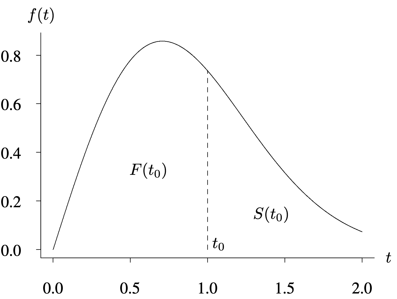
Mathematically, this means the survival function is the integral of the density function from $t$ to infinity:

Conversely, the density function $f(t)$ is the negative of the derivative (the slope) of the survival function. Intuitively, this means that when the probability of survival $S(t)$ is dropping quickly, the failure density $f(t)$ must be high.

The Central Equation: Connecting Hazard, Density, and Survival

In the previous lesson, you were introduced to the foundational formula that connects three of our key functions. Let's formalize it. The hazard function is defined as the ratio of the probability density function to the survival function.

This equation is elegant and powerful. It tells us that the instantaneous risk at time $t$ ($h(t)$) is the likelihood of failure at that instant ($f(t)$) adjusted for the proportion of individuals who are still alive and able to experience the event ($S(t)$). A high failure density doesn't necessarily mean a high hazard if very few individuals have survived to that point.

This definition is clearly laid out in the following textbook section.

From Hazard to Survival: The Power of Accumulated Risk

The most useful relationship in practice is the one that connects the hazard function back to the survival function. This allows us to model risk directly and then see its implications for survival probability. This involves the cumulative hazard function, $H(t)$.

Recall that $H(t)$ is the total accumulated risk up to time $t$. If you think of $h(t)$ as a "risk curve," $H(t)$ is the area under that curve from the beginning up to time $t$.

The fundamental relationship that connects this accumulated risk back to survival is:

This equation tells us that the probability of surviving past time $t$ is the exponential of the negative accumulated hazard. A large accumulated hazard leads to an exponentially smaller probability of survival. This exponential relationship is a cornerstone of survival analysis.

Because $H(t)$ is the integral of $h(t)$, we can also write this as:

The following video provides an excellent walkthrough of how these functions are related through calculus, but explains it in a very accessible way. It culminates in deriving the link between the cumulative hazard and survival functions.

The "Rosetta Stone" of Survival Functions

We've now established the key links. The wonderful thing is that if you know any one of the four functions, you can derive all the others. The textbook provides a handy table that summarizes all of these transformations. It's like a "Rosetta Stone" for converting between the different representations of a lifetime distribution.

Let's see this in action with a simple, concrete example: the exponential distribution. This distribution is defined by having a constant hazard, $h(t)=\lambda$. This means the risk of the event is the same at all times, a "memoryless" process.

What do the other functions look like? We can use the relationships from Table 4.1.

1. Given: $h(t)=\lambda$
2. Find Cumulative Hazard $H(t)$: We integrate the hazard. The area under a constant line is just the height times the length. $$H(t)={\int }_0^t\lambda dx=\lambda t$$ The accumulated risk grows linearly with time.
3. Find Survival Function $S(t)$: We use our key formula. $$S(t)=\exp (-H(t))=\exp (-\lambda t)$$ Survival probability decays exponentially.
4. Find Density Function $f(t)$: We can use $f(t)=h(t)\times S(t)$. $$f(t)=\lambda \times \exp (-\lambda t)$$ This is the classic probability density function for the exponential distribution.

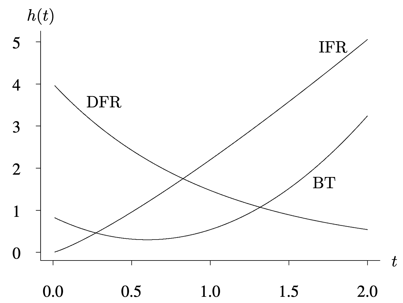
This simple example shows how the entire system works together, starting from a single assumption about the nature of the risk. Different assumptions about the shape of the hazard function (e.g., increasing or decreasing) will generate different families of distributions.

Conclusion

In this lesson, we have cemented the theoretical foundation of survival analysis by formalizing the links between its four key functions.

Key Takeaways:

• The probability density $f(t)$, survival $S(t)$, hazard $h(t)$, and cumulative hazard $H(t)$ functions are four equivalent representations of a time-to-event distribution.
• Knowing any one of these functions allows you to mathematically derive the other three.
• The two most critical relationships to understand are:
  1. The definition of hazard: $h(t)=\frac{f(t)}{S(t)}$
  2. The link between accumulated hazard and survival: $S(t)=\exp (-H(t))$

With this theoretical framework in place, you are now equipped to understand how survival models work from the ground up.

In our next lesson, we will shift from theory to application. We will learn how to estimate the survival function directly from a real-world dataset, even when our observations are incomplete due to censoring. This will introduce you to one of the most famous and widely used tools in survival analysis: the Kaplan-Meier estimator.