Kaplan-Meier Survival Analysis

Introduction

In our last lesson, we established the core theoretical relationships connecting the survival, hazard, density, and cumulative hazard functions. We saw how assuming a specific mathematical form for the hazard—like a constant rate in the exponential distribution—allows us to derive a smooth, theoretical survival curve.

But what happens in the real world, where data is messy and we often don't know the true underlying distribution? How can we estimate the survival function directly from observational data, especially when that data includes censored observations? This lesson introduces the Kaplan-Meier estimator, a cornerstone of survival analysis that addresses this exact problem. It is a powerful non-parametric method, meaning it doesn't require us to assume a specific distribution for survival times. Your goal for this lesson is to learn how to estimate a survival function from censored data by applying the step-by-step logic of the Kaplan-Meier method.

The Problem with Simple Proportions

Imagine you are tracking 10 patients, and at the end of one year, 8 are still alive. You might be tempted to say the one-year survival rate is 8/10 or 80%. But what if one of those 8 patients was lost to follow-up at 6 months? We know they survived at least 6 months, but we don't know what happened after. Simply excluding them or counting them as "survived" at one year would be incorrect and waste valuable information.

The Kaplan-Meier method provides an elegant solution by reframing the question. Instead of calculating a single proportion at the end, it calculates the probability of surviving through a series of time intervals, and then multiplies these probabilities together.

The Core Idea: A Chain of Conditional Probabilities

The fundamental insight of the Kaplan-Meier method is that the probability of surviving past a certain time $t$ is the product of the probabilities of surviving each preceding interval where an event occurred.

Let's say events happen at times $t_{1}, t_{2}, \dots, t_{k}$ . The survival probability at time $t_{k}$ can be thought of as:

The probability of surviving past $t_{1}$ .
Times the probability of surviving past $t_{2}$ , given you survived past $t_{1}$ .
Times the probability of surviving past $t_{3}$ , given you survived past $t_{2}$ .
...and so on, up to $t_{k}$ .

This chain of conditional probabilities is the key. The following video explains this concept of cumulative probability very intuitively.

Kaplan Meier curve and hazard ratio tutorial (Kaplan Meier curve and hazard ratio made simple!)

This video from Eric McCoy provides a clear, conceptual walkthrough of how a survival curve is built by multiplying probabilities from one interval to the next.

Watch the segment from the start of the curve construction. Pay close attention to how the speaker explains the "cumulative probability" at each step as a product of the previous survival probability and the current "interval probability." This is the core logic we will be using.

To formalize this, we need two key pieces of information at each event time $t_{i}$ :

$n_{i}$ : The number of individuals who are "at risk" of the event just before time $t_{i}$ . This includes everyone who has not yet had the event or been censored.
$d_{i}$ : The number of individuals who experience the event at time $t_{i}$ .

The conditional probability of surviving past time $t_{i}$ is then $(n_{i} - d_{i}) / n_{i}$ . The Kaplan-Meier estimator is the product of these conditional probabilities for all event times up to and including time $t$ .

The formula is written as:

S (t) = i ∣ t_{i} \leq t \prod \frac{n _{i} - d _{i}}{n _{i}}

Here, the $\prod$ symbol is the product operator, meaning you multiply the term $(n_{i} - d_{i}) / n_{i}$ for all event times $t_{i}$ that have occurred up to time $t$ .

Kaplan-Meier Estimator: Practical Guide for Data-Driven Decisions ...

This article from MCP Analytics clearly states the mathematical foundation of the estimator and explains how it incorporates censored data.

Please read the section titled How the Kaplan-Meier Estimator Works. Focus on the formula provided under the heading and the subsequent explanation of how the "at risk" count, n_i, is defined.

The Kaplan-Meier Algorithm: A Step-by-Step Calculation

Given your background in information systems, it's useful to think of the Kaplan-Meier calculation as a step-by-step algorithm. Let's walk through it using a small dataset.

Here is the data from the GraphPad resource, representing 20 participants. Event=1 means the event occurred; Event=0 means the observation was censored.

Participant	Time	Event
03	1	1
08	1	0
02	2	1
05	2	0
06	2	1
...	...	...
07	6	1

The full process is detailed in the following guide. We will break it down together.

The mathematics of Kaplan-Meier survival analysis - GraphPad

This guide from GraphPad provides an exceptionally clear, manual walkthrough of the entire Kaplan-Meier calculation from raw data to the final plot.

Read through the entire article. We will summarize the key steps below. Pay close attention to the "life table" and how the Number at risk, Number of events, and Survival probability are calculated at each time point. Notice specifically how the Number at risk for the next time point is calculated.

Let's reconstruct the logic from the GraphPad article.

Step 1: Order the Data
First, order all observations by their follow-up time, from smallest to largest. This gives us a timeline of all events and censoring points.

Step 2: Create a "Life Table"
We build a table to track the calculation. The essential columns are:

Time (t): The unique time points where at least one event occurred.
Number at Risk (n): The number of subjects still in the study just before time t.
Number of Events (d): The number of events that happened at exactly time t.
Number Censored (c): The number of subjects censored at time t.
Survival Probability S(t): The estimated cumulative survival.

Step 3: Iterate and Calculate

At Time 0: The survival probability $S (0)$ is 1 (or 100%). The number at risk is the total number of participants, $n_{0} = 20$ .
At the first time point, t=1:
- From the data, we see one event ( $d_{1} = 1$ ) and one censored observation ( $c_{1} = 1$ ).
- The number at risk, $n_{1}$ , is still 20, because these individuals were at risk just before time 1.
- The conditional probability of surviving past t=1 is $(n_{1} - d_{1}) / n_{1} = (20 - 1) /20 = 0.95$ .
- The cumulative survival is $S (1) = S (0) \times 0.95 = 1 \times 0.95 = 0.95$ .
Prepare for the next time point, t=2:
- This is the crucial step where censoring is handled. The number at risk for the next interval, $n_{2}$ , is the previous number at risk minus those who had the event AND those who were censored.
- $n_{2} = n_{1} - d_{1} - c_{1} = 20 - 1 - 1 = 18$ .
At t=2:
- From the data, there are five events ( $d_{2} = 5$ ) and one censored observation ( $c_{2} = 1$ ) at time 2.
- The number at risk is $n_{2} = 18$ .
- The conditional probability of surviving past t=2 is $(n_{2} - d_{2}) / n_{2} = (18 - 5) /18 \approx 0.722$ .
- The new cumulative survival is $S (2) = S (1) \times 0.722 = 0.95 \times 0.722 \approx 0.686$ .

This process continues until the last observation. The image below, taken from the numiqo video, provides a fantastic visual summary of this iterative calculation.

This table shows a numerical example of the Kaplan-Meier calculation. For each time point, it lists the number of events (m), censored observations (q), and the number at risk (n). The survival probability S(t) is calculated iteratively by multiplying the previous survival probability by the conditional probability of survival at the current step, which is (n-m)/n.

The video this image is from also provides a great narrated walkthrough of the calculation.

Kaplan-Meier-Curve [Simply Explained]

This video by numiqo visually demonstrates the step-by-step calculation of the survival probabilities when censored data is present.

Please watch the segment from where censored data is introduced. The presenter shows how to fill out the table and perform the iterative multiplication to get the final survival probabilities. Note that their notation is slightly different: m is events (d), q is censored (c), and n is number at risk.

Visualizing and Interpreting the Kaplan-Meier Curve

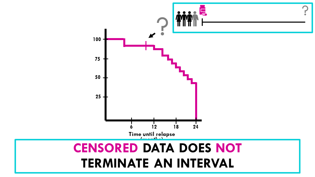
Once the life table is complete, we plot Time (t) on the x-axis and Survival Probability S(t) on the y-axis. The result is a characteristic "stair-step" curve.

This is a typical Kaplan-Meier curve. The y-axis shows survival probability, and the x-axis shows time. The curve only drops when an event occurs. The small tick mark on the curve indicates a censored observation. Notice that censoring does not cause a drop in the survival probability; the person simply stops contributing to the 'at risk' pool for subsequent calculations.

Key features to remember when interpreting the curve:

The curve begins at 1 (100% survival).
Horizontal lines represent intervals where no events occurred. Survival probability remains constant.
Vertical drops occur only at the time of an event. The size of the drop depends on the number of events relative to the number of people at risk at that time. A larger drop means a higher proportion of the at-risk group experienced the event.
Tick marks (or other symbols) on the curve represent censored observations. They signify that individuals have been removed from the risk set, but they do not cause the survival probability to decrease. This is a critical point: censored data does not terminate an interval.

The main takeaway from the curve is often the median survival time, which is the time at which the survival probability $S (t)$ drops to 0.5 (50%). This represents the time by which half of the study population has experienced the event.

Conclusion

In this lesson, we moved from the abstract theory of survival functions to the practical, algorithmic method for estimating them from real-world data. The Kaplan-Meier estimator is a fundamental tool that you will encounter frequently in epidemiological and clinical research.

Key Takeaways:

The Kaplan-Meier method is a non-parametric approach to estimate the survival function from time-to-event data.
Its main strength is its ability to correctly incorporate censored observations.
The survival probability is calculated as a product of conditional probabilities at each event time.
The calculation follows a clear, step-by-step process of creating a "life table" and iterating through the event times.
Censored subjects are removed from the "number at risk" for subsequent time points but do not cause a drop in the survival curve themselves.

Now that you can estimate a survival curve for a single group, a natural question arises: what if we have two groups, such as a treatment and a control group, and we want to compare their survival? In our next lesson, we will learn how to use the log-rank test to formally determine if the difference between two or more Kaplan-Meier curves is statistically significant.