Comparing Survival Curves with the Log-Rank Test

Introduction

In our previous lesson, we mastered the Kaplan-Meier method to estimate and visualize a survival curve for a single group, even when faced with censored data. This was a crucial step in understanding the survival experience of a population. However, in epidemiology and clinical trials, we are rarely interested in just one group. More often, we want to compare outcomes between different groups—for example, patients receiving a new drug versus those on a placebo, or smokers versus non-smokers.

This lesson directly addresses that need. We will learn how to formally compare survival distributions between two or more groups using the log-rank test. By the end of this lesson, you will be able to look at two Kaplan-Meier curves, apply the log-rank test, and interpret its result to determine whether the observed differences in survival are statistically significant or likely due to random chance.

The Question: Are the Survival Curves Really Different?

Imagine we have two groups of patients in a study, and we plot their Kaplan-Meier curves on the same graph. One curve might appear to be consistently above the other, suggesting better survival. But how can we be sure this difference isn't just a fluke of our particular sample? We need a formal statistical method to answer this question.

The log-rank test is a non-parametric hypothesis test designed for this exact purpose. It allows us to test whether the survival distributions of two or more independent groups are identical.

Like any hypothesis test, it operates with a null and an alternative hypothesis.

This image illustrates the core question of the log-rank test. The null hypothesis assumes the groups have identical survival curves, while the alternative hypothesis proposes that their curves are different.

Null Hypothesis (H₀): There is no difference in the survival distributions among the groups. In the overall population, the survival curves are identical. Any difference we see in our sample data is due to random variation. Mathematically, for two groups, this is written as $S_{1} (t) = S_{2} (t)$ for all time points $t$ .
Alternative Hypothesis (H₁): The survival distributions are different. At least one group has a survival experience that is systematically different from the others. Mathematically, $S_{1} (t) \neq = S_{2} (t)$ for at least some time $t$ .

The log-rank test calculates a p-value to help us decide between these two hypotheses. The following reading provides a concise summary of the test's purpose and how to interpret its result.

Easy log rank test for survival analysis - biostatsquid.com

This article from Biostatsquid gives a clear, high-level overview of the log-rank test, its hypotheses, and the interpretation of its p-value.

Read the article from the beginning down to the end of the section "How to interpret log rank test results". Pay close attention to the sections defining what the test does, the formal statement of the null and alternative hypotheses, and the rules for interpreting the p-value.

As a quick review: if the p-value is less than our chosen significance level (typically 0.05), we reject the null hypothesis and conclude that there is a statistically significant difference between the survival curves. If the p-value is greater than 0.05, we fail to reject the null hypothesis, meaning we do not have sufficient evidence to conclude that the curves are different.

The Intuition: Comparing Observed vs. Expected Events

So, how does the log-rank test actually arrive at this p-value? The core logic is elegant and, given your background, can be thought of as an algorithm that iterates through the data. It compares the number of events we actually saw in each group to the number of events we would have expected if the null hypothesis were true.

Let's break this down. The test proceeds by looking at every time point where at least one event (e.g., death) occurred.

Pool the Data: At a specific event time, we momentarily ignore the group assignments and look at the total number of people at risk and the total number of events across all groups combined. This gives us the overall event rate at that instant.
Calculate Expected Events: Assuming the null hypothesis is true (i.e., survival is the same for everyone regardless of group), we calculate the expected number of events in each group. This expected count is simply the overall event rate multiplied by the number of people at risk in that specific group. For instance, if Group A has 30 people at risk and Group B has 10 (total 40), and 4 events occur, we'd expect 75% of those events (3 events) to be in Group A and 25% (1 event) in Group B.
Compare Observed and Expected: We then compare this expected number to the observed number of events that actually happened in each group at that time.
Sum the Discrepancies: The test statistic is essentially built by summing the differences (Observed - Expected) across all the event times for each group.
Calculate the Test Statistic: These summed differences are used to compute a chi-square ( $χ^{2}$ ) statistic. A large $χ^{2}$ value indicates a big discrepancy between what we observed and what we expected under the null hypothesis, leading to a small p-value.

The following video provides an excellent intuitive explanation of this entire process, framing the log-rank test as a chi-square test that compares observed and expected counts.

LOG RANK TEST for survival analysis - easily explained with an example!

This video from the Biostatsquid channel wonderfully explains the logic and interpretation of the log-rank test without getting lost in complex formulas.

Please watch from the beginning until the end of the intuitive explanation. Focus on these key segments: The Purpose of the Test: This sets the stage with a clear clinical trial example. Hypotheses and P-values: This reinforces the hypothesis testing framework and how to interpret the results. Observed vs. Expected: This is the core of the video, where the speaker explains how the test works by comparing observed events to the expected number of events under the null hypothesis.

A Look at the Calculation

While statistical software will perform the calculation for us, seeing the mechanics step-by-step can solidify your understanding. The process involves creating a contingency table for each event time.

The Stats and R article provides a complete, manual walkthrough of a log-rank test calculation. We won't focus on memorizing the formulas, but rather on understanding how the table is constructed to get the final test statistic. This algorithmic approach should feel familiar.

What is survival analysis? Examples by hand and in R - Stats and R

This article shows how to perform the log-rank test by filling out a table, column by column. This makes the calculation very transparent.

Start at the section Log-rank test. Read the brief introduction and the statement of the hypotheses. Then, focus on the subsection "By hand". Follow the step-by-step description of how to fill in each column of the table. Try to connect the column definitions to the concepts we just discussed: d_j1 and d_j2 are the observed event counts in each group at time y_j. E_j is the expected event count in group 1 at that time, calculated using the proportion of individuals at risk in that group (R_j1 / R_j). The O_j - E_j column shows the discrepancy at each step. Finally, see how these values are summed and used to compute the final test statistic and p-value.

The final test statistic from this process is compared to a chi-square distribution to obtain the p-value.

Interpreting the Results in Context

Let's look at a complete example. The plot below shows two Kaplan-Meier curves and the p-value from a log-rank test comparing them.

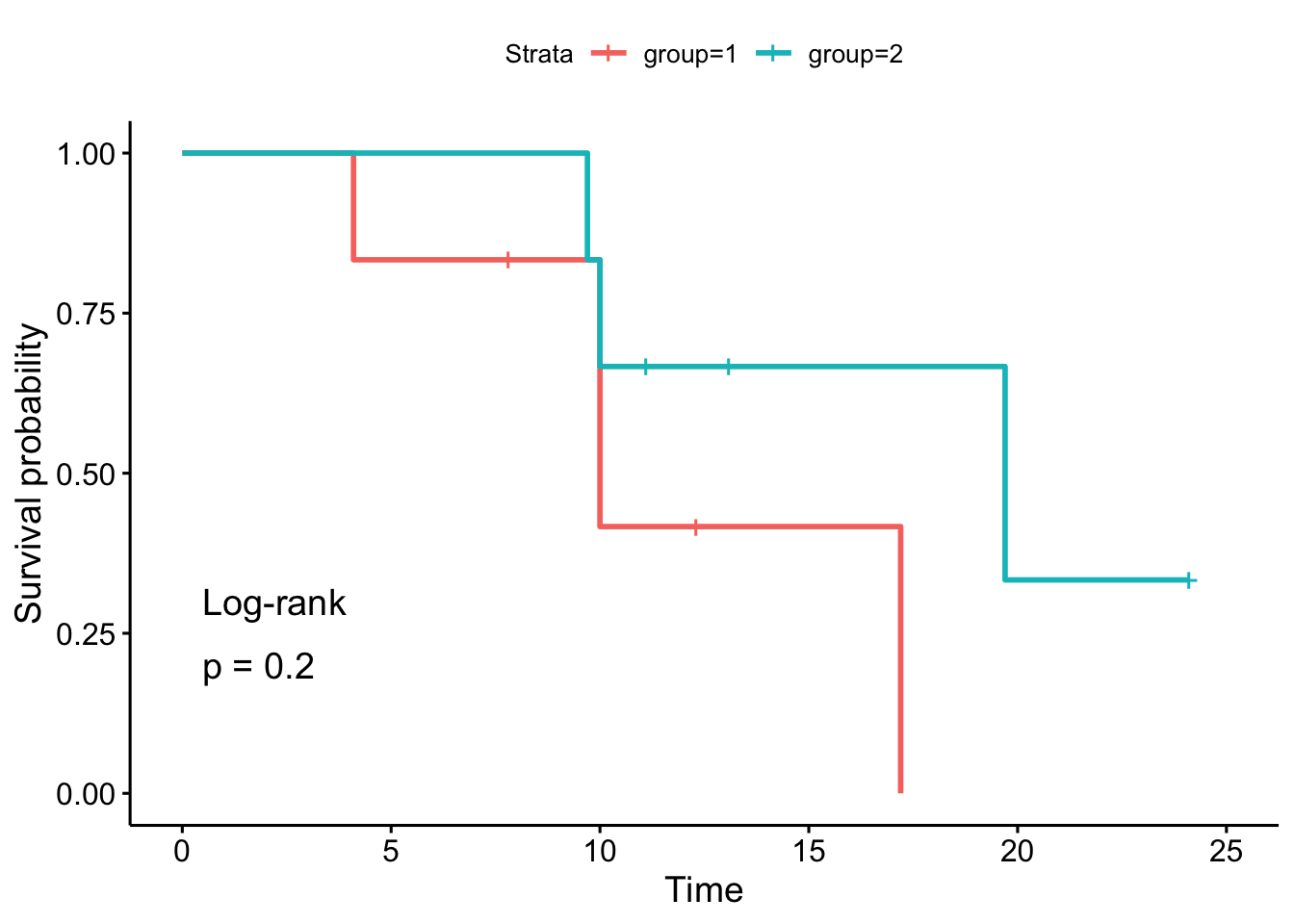
Kaplan-Meier survival curves for two groups. The log-rank test yields a p-value of 0.2, which is used to assess the statistical significance of the difference between the two survival distributions.

In this plot:

We see two survival curves, one for group=1 (red) and one for group=2 (blue). Visually, the red curve drops faster, suggesting poorer survival.
The log-rank test gives a p = 0.2.
Since 0.2 is greater than the standard threshold of 0.05, we fail to reject the null hypothesis.
Conclusion: Despite the visual difference between the curves, we do not have enough statistical evidence from this sample to conclude that there is a true difference in the survival distributions of group 1 and group 2 in the wider population. The observed difference could plausibly be due to random chance.

Limitations and the Path Forward

The log-rank test is a powerful tool, but it has two key limitations:

It doesn't measure the size of the effect. It gives us a p-value that answers "Is there a difference?" but it doesn't tell us how big that difference is (e.g., is one group's risk of death twice as high as the other?).
It cannot adjust for other variables. In our examples, we only compared groups based on one factor (e.g., treatment A vs. B). What if the groups also differ in age, disease severity, or other factors that could influence survival? The log-rank test cannot account for these potential confounders.

These limitations lead us directly to the next major topic in survival analysis: regression modeling. Models like the Cox proportional hazards model (which we'll cover in Module 7) can estimate the magnitude of the difference (the hazard ratio) while simultaneously adjusting for multiple other variables.

Conclusion

In this lesson, we completed our foundational toolkit for non-parametric survival analysis. We learned how to go from generating individual survival curves with the Kaplan-Meier estimator to formally comparing them using the log-rank test.

Key Takeaways:

The log-rank test is used to statistically compare the survival distributions of two or more independent groups.
The null hypothesis (H₀) is that the survival curves are identical across groups.
The test works by comparing the observed number of events in each group to the expected number of events, assuming H₀ is true.
The result is a p-value, which tells us the probability of observing a difference as large as we did (or larger) if there were truly no difference between the groups.
A small p-value (< 0.05) allows us to reject H₀ and conclude the survival distributions are significantly different.
The log-rank test tells us if there's a difference, but not how large it is or how to adjust for other factors.

This lesson concludes our module on the fundamentals of survival analysis. We've covered time-to-event data, censoring, the core functions (S(t) and h(t)), Kaplan-Meier estimation, and the log-rank test. You now have the theoretical basis to understand and interpret the most common non-parametric methods used in survival studies. In the next module, we will explore a different approach: parametric survival models, where we assume the survival times follow a specific statistical distribution like the exponential or Weibull distribution.

Recommended resources