Survival and Hazard Functions

The Survival Function: Quantifying "Event-Free" Time

The most direct way to describe the outcome in a time-to-event study is by tracking the proportion of a population that remains free of the event over time. This is precisely what the survival function does.

The survival function, denoted as $S(t)$, is the probability that the time-to-event, $T$, is greater than some specified time $t$.

In simple terms, it's the probability of "surviving" past time $t$. The "event" doesn't have to be death; it could be machine failure, disease recurrence, or customer churn.

• At the start of the study ($t=0$), no one has experienced the event, so $S(0)=1$.
• As time progresses, individuals experience the event, so the probability of survival can only decrease or stay the same. Therefore, $S(t)$ is a non-increasing function.
• Theoretically, if you follow the population long enough, everyone will experience the event, and the survival function will approach $S(\infty )=0$.

The following video provides an excellent visual introduction to the survival function and its relationship to the cumulative distribution function (which tracks the proportion who have experienced the event).

To solidify this definition, let's look at a more formal description.

As the text mentions, the survival function $S(t)$ is also called the reliability function in engineering or the complementary cumulative distribution function, since $S(t)=1-F(t)$, where $F(t)$ is the probability of the event happening by time $t$.

The Hazard Function: The Instantaneous Risk

While the survival function tells us about the overall probability of remaining event-free, the hazard function, $h(t)$, gives us a more dynamic, moment-to-moment measure of risk.

The hazard function, $h(t)$, represents the instantaneous potential for an event to occur at time $t$, given that the individual has survived up to time $t$.

This conditional nature is the most important concept to grasp. The hazard is not the overall probability of failure at time $t$; it's the risk at time $t$ for those still at risk at that moment.

Think back to our speedometer analogy. The hazard function is the "risk speedometer." It tells you how high the risk is at any specific instant. Because it's a rate (events per unit of time), its value is not bounded between 0 and 1; it can be greater than 1.

The video below gives an excellent explanation of this conditional concept and how the hazard function is calculated and interpreted.

Interpreting the Shape of the Hazard Function

The real power of the hazard function comes from its shape over time, which tells a story about the nature of the risk. Different processes have characteristically different hazard shapes.

1. Increasing Hazard (Curve 2): The risk of the event increases over time. This is typical of "wear-out" phenomena. The risk of engine failure in a car increases as it ages. For humans, the risk of death from age-related disease increases throughout adulthood. This is often called an Increasing Failure Rate (IFR).

2. Decreasing Hazard (Curve 4): The risk of the event is highest at the beginning and decreases over time. This pattern is common in post-surgical survival, where the immediate post-operative period is riskiest. In your field of computer information systems, this is analogous to software bugs: many bugs are found and fixed shortly after a new release, so the "hazard" of encountering a critical bug decreases as the software matures. This is known as a Decreasing Failure Rate (DFR).

3. Constant Hazard (Curve 3): The risk of an event is the same at all times, regardless of how long an item has survived. This implies a "memoryless" process. An example is the decay of a radioactive atom; its probability of decaying in the next second is constant, no matter how long it has already existed. This corresponds to the Exponential distribution, a key model in survival analysis.

4. Bathtub Shape (Curve 1): This is a composite shape. There's an initial period of high risk due to "infant mortality" or manufacturing defects (decreasing hazard). This is followed by a period of low, relatively constant risk. Finally, risk begins to increase due to wear-out (increasing hazard). This is a very common model for human lifetimes and for the reliability of complex electronic or mechanical systems.

The following text provides more detail on these hazard shapes and their real-world applications.

The Relationship Between Survival and Hazard

The survival and hazard functions are two sides of the same coin. They are intrinsically linked: a higher hazard rate will cause the survival probability to decrease more rapidly.

• When the hazard $h(t)$ is high, the survival curve $S(t)$ will be steep.
• When the hazard $h(t)$ is low, the survival curve $S(t)$ will be relatively flat.

The following graph shows this relationship clearly.

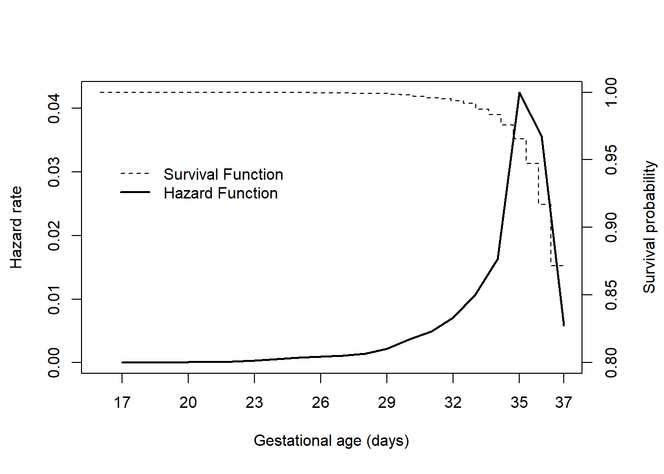
As you can see, the survival probability remains very high and stable while the hazard rate is close to zero. As the hazard rate increases, indicating a rising risk of the event, the survival curve begins to slope downwards more steeply.

Conclusion

In this lesson, we have formally defined the two most important functions for describing time-to-event data.

Key Takeaways:

• The Survival Function $S(t)$ gives the probability of remaining event-free beyond time $t$. It is a probability, ranging from 1 down to 0, and is always non-increasing.
• The Hazard Function $h(t)$ represents the instantaneous risk of an event at time $t$, conditional on having survived up to that point. It is a rate (not a probability) and its shape over time (increasing, decreasing, constant, etc.) reveals the nature of the risk.
• The two functions are inversely related: a higher hazard leads to a more rapid decline in survival.

We have now defined the core concepts needed to model survival data: the survival function $S(t)$ to describe outcomes, and the hazard function $h(t)$ to describe risk. In our next lesson, we will complete this foundational picture by exploring the precise mathematical relationships that link $S(t)$, $h(t)$, the probability density function $f(t)$, and the cumulative hazard function $H(t)$. This will equip you with a complete theoretical framework for understanding survival models.