The Integral as Accumulated Hazard

From Instantaneous Rate to Total Accumulation

In the previous lesson, we established that the hazard function, $h(t)$, tells us the risk at a precise moment in time. But how do we describe the total risk an individual has faced up to a certain point? For example, what is the total burden of risk for a patient two years after surgery?

To answer this, let's return to our car analogy.

• The speedometer shows your speed right now (the rate of change of distance). This is the derivative.
• The odometer shows the total distance you have traveled since you started your trip.

How does the odometer calculate this total distance? Conceptually, it continuously adds up all the small distances traveled in every tiny interval of time. If you travel at 60 mph for one hour, you cover 60 miles. If your speed varies, the odometer is essentially summing up the distance covered in each second (or millisecond) to get the grand total.

In calculus, this process of summing up a quantity that changes over time is called integration. The integral of a rate function (like speed) over a time period gives you the total accumulated quantity (like distance). Visually, if you plot speed versus time, the total distance traveled is the area under the curve.

Introducing the Cumulative Hazard Function

Now, let's apply this logic to survival analysis.

• The hazard function, $h(t)$, is our "speedometer" of risk.
• The cumulative hazard function, $H(t)$, is our "odometer" of risk. It measures the total, accumulated risk an individual has been exposed to from the beginning (time 0) up to time $t$.

The following video from zedstatistics provides a great introduction to this idea, framing the cumulative hazard as the area under the hazard function curve.

As the video explains, the cumulative hazard, often denoted as a capital $H(t)$, is the integral of the hazard function $h(t)$ from time 0 to $t$:

You don't need to perform the integration yourself, but it's crucial to understand what it represents: $H(t)$ is the sum of all the instantaneous risks from the start of follow-up until time $t$.

The article below offers another excellent, non-technical explanation that distinguishes between the instantaneous risk given by the hazard function and the total accumulated risk given by the cumulative hazard function.

Interpreting the Cumulative Hazard

The value of the cumulative hazard function, $H(t)$, can be thought of as the total "burden of risk" or the expected number of events if the event could happen multiple times to one individual. For example, if $H(t=2\text{ years})=0.5$, it represents the total amount of risk the subject has accumulated over those two years. A higher value means a greater cumulative risk exposure.

A key property of the cumulative hazard function is that it is always non-decreasing. While the instantaneous risk, $h(t)$, can go up or down over time, the total accumulated risk can only increase or stay the same. You can't "un-accumulate" risk.

This relationship is shown perfectly in the image below.

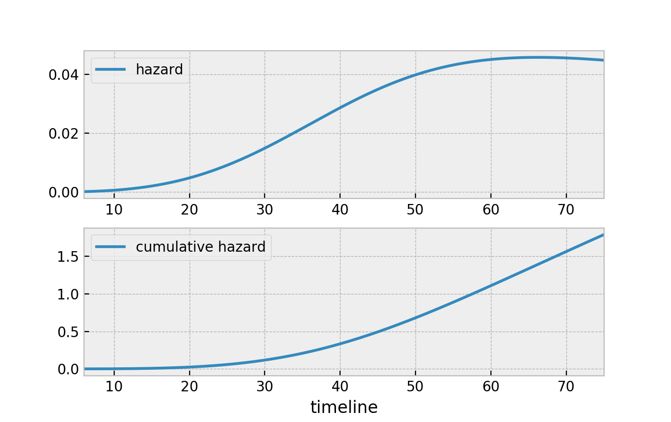
In the "Hazard and Cumulative Hazard Functions" image, observe the top panel where the hazard rate increases until about t=60 and then slightly decreases. Now look at the bottom panel. The cumulative hazard curve is steepest when the hazard rate is highest (from t=30 to t=60), indicating risk is accumulating fastest. When the hazard rate decreases after t=60, the cumulative hazard curve continues to rise, but less steeply. It never goes down.

To formalize this, let's look at the definition from the textbook chapter we consulted previously.

The Central Role of the Cumulative Hazard

You might be wondering why this concept is so important. The cumulative hazard function, $H(t)$, acts as a critical bridge between the instantaneous hazard rate, $h(t)$, and the most intuitive measure in survival analysis: the survival function, $S(t)$. As we will see in the next lesson, there is a direct mathematical relationship that allows us to calculate the probability of survival up to a certain time if we know the total accumulated risk up to that time.

The diagram below provides a roadmap of how all these concepts connect. We've now discussed the Hazard and the Cumulative Hazard. Soon, we will see how they link directly to the Survival function and the other components.

For now, focus on the arrow leading from "Hazard" to "Cumulative Hazard" labeled with an integral sign (${\int }_0^t\cdot ds$). This is the process we've discussed today: accumulating instantaneous risk over time to find the total risk.

Conclusion

In this lesson, we bridged the gap from instantaneous rates to total accumulation using the concept of the integral.

Here are the key takeaways:

• The integral of a rate over a period gives the total accumulated amount, equivalent to the area under the curve of the rate's graph.
• In survival analysis, integrating the hazard function $h(t)$ gives us the cumulative hazard function $H(t)$.
• $H(t)$ represents the total accumulated risk or "burden of risk" from time 0 up to time $t$.
• Unlike the hazard function, the cumulative hazard function is always non-decreasing.

We have now defined risk both at an instant ($h(t)$) and as an accumulation over time ($H(t)$). In our next lesson, we will put these pieces together to formally define the survival and probability density functions and explore the precise mathematical relationships between them, as mapped out in the diagram you just saw. This will complete our foundational toolkit for modeling time-to-event data.