Interpreting Logistic Regression Coefficients

From Straight Lines to S-Curves

Imagine we want to model the probability of a person having coronary heart disease (CHD) based on their age. The outcome is binary (CHD: yes=1, no=0), and the probability must be between 0 and 1. If we try to fit a simple linear regression line, it might predict probabilities less than 0 for very young people or greater than 1 for very old people, which is nonsensical.

To solve this, we need a function that takes any linear combination of predictors and "squishes" the output into the [0, 1] range. The function that does this is the logistic function, which produces a characteristic S-shaped curve (a sigmoid curve).

However, to build our model, we do something clever. Instead of modeling the probability directly, we transform it in a way that allows us to use a linear equation, just like in the last lesson. This transformation involves two steps: from probability to odds, and from odds to log-odds.

The Logit Transformation: From Probability to Log-Odds

Let's break down these essential concepts.

1. Probability (p): The likelihood of an event occurring, ranging from 0 to 1.
2. Odds: The ratio of the probability of an event happening to the probability of it not happening.
   $\text{Odds}=\frac{p}{1-p}$
   For example, if the probability of having a disease is 0.2 (20%), the odds are $0.2/(1-0.2)=0.2/0.8=0.25$. We can say the odds are "1 to 4". Unlike probability, odds range from 0 to positive infinity.
3. Log-Odds (or Logit): The natural logarithm of the odds.
   $\text{Log-Odds}=\ln \left(\frac{p}{1-p}\right)$
   Taking the logarithm of the odds transforms the scale from [0, +∞) to (-∞, +∞). This is the crucial step! Because the log-odds are unbounded, we can now model them with a simple linear equation. This transformation is called the logit link function.

The following reading explains this transformation very clearly.

The StatQuest video below gives a fantastic visual intuition for how this logit transformation converts the S-shaped logistic curve into a straight line, which is why we can apply a linear model to it.

The Logistic Regression Model and Its Coefficients

With the logit transformation, the logistic regression model looks strikingly similar to the linear regression model:

Here:

• The left side is the log-odds of the outcome.
• The right side is a linear equation with an intercept (${\beta }_0$) and a slope (${\beta }_1$) for our predictor variable $X$.

The coefficients (${\beta }_0$ and ${\beta }_1$) are estimated from the data, typically using a method called maximum likelihood estimation (which we will cover in a later lesson). Our focus now is on what these coefficients mean once we have them.

There are three primary ways to interpret the coefficients, as summarized in the infographic below. We will focus on the last two, as they are the most useful.

Interpretation 1: The Log-Odds (The "Raw Math")

The most direct interpretation is in terms of log-odds.

• ${\beta }_1$: For a one-unit increase in $X$, the log-odds of the outcome is expected to change by ${\beta }_1$.
• ${\beta }_0$: This is the log-odds of the outcome when $X=0$.

While mathematically correct, "log-odds" are not very intuitive for most people. Therefore, we typically take one more step and convert the log-odds back into a more understandable scale: the odds ratio.

Interpretation 2: The Odds Ratio (The Most Common Method)

To get from log-odds back to odds, we use the inverse of the natural logarithm, which is exponentiation (i.e., raising $e$ to the power of the coefficient).

The odds ratio (OR) is calculated as $e^{{\beta }_1}$ or $\exp ({\beta }_1)$.

• $\exp ({\beta }_1)$: For a one-unit increase in $X$, the odds of the outcome are multiplied by a factor of $\exp ({\beta }_1)$.

How to interpret the odds ratio value:

• If OR > 1, the odds of the outcome increase as $X$ increases. For example, an OR of 1.5 means the odds increase by 50% for each one-unit increase in X.
• If OR < 1, the odds of the outcome decrease as $X$ increases. For example, an OR of 0.8 means the odds decrease by 20% (or are 80% of the original odds) for each one-unit increase in X.
• If OR = 1, there is no association between $X$ and the odds of the outcome.

The following resource provides a clear walkthrough of this interpretation.

Examples of Interpretation

Let's apply this to a concrete example from an epidemiological study. The image below shows the output of a logistic regression analysis estimating the risk of cardiovascular disease (CVD) for people who are obese.

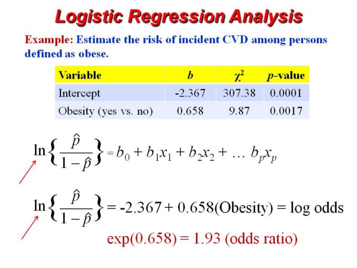
Let's interpret the coefficient for the Obesity variable, which is ${\beta }_1=0.658$.

1. As Log-Odds: The log-odds of having CVD for an obese person is 0.658 higher than for a non-obese person.

2. As an Odds Ratio: We exponentiate the coefficient: $\exp (0.658)\approx 1.93$.

   • Interpretation: The odds of having CVD are 1.93 times higher for obese individuals compared to non-obese individuals.
   • Alternatively, we can say that the odds of having CVD are 93% higher for obese individuals.

The following video provides more excellent examples of interpreting coefficients for both continuous and categorical predictor variables.

A Crucial Distinction: Odds vs. Probability

It is extremely common for people to misinterpret an odds ratio as a "risk ratio" or to say that the probability increases by a certain percentage. This is incorrect. An odds ratio of 2.0 does not mean the probability of the outcome doubles.

The relationship between odds and probability is non-linear. A change in odds has a different impact on probability depending on the starting point. If the baseline probability is low, a change in odds results in a similar change in probability. However, if the baseline probability is high, the same change in odds will have a much smaller effect on the probability.

Conclusion

In this lesson, you have learned the fundamental theory and practical interpretation of logistic regression, a cornerstone of modern epidemiology and biostatistics.

Here are the key takeaways:

• Logistic regression is used to model binary outcomes (0/1, yes/no).
• It works by modeling the log-odds of the outcome as a linear function of the predictor variables: $\ln (p/(1-p))={\beta }_0+{\beta }_{1}X$.
• A regression coefficient (${\beta }_1$) represents the change in the log-odds of the outcome for a one-unit change in the predictor.
• The odds ratio ($\exp ({\beta }_1)$) is a more intuitive measure. It represents the multiplicative factor by which the odds of the outcome change for a one-unit change in the predictor.
• An odds ratio is not the same as a probability or risk ratio, and this distinction is crucial for correct interpretation.

We have now covered the two most fundamental regression models: linear for continuous outcomes and logistic for binary outcomes. In our next lesson, we will formally define epidemiology and explore the core measures of disease frequency—incidence and prevalence—that are often the outcomes we seek to model with these powerful statistical tools.