Interpreting Regression Coefficients and R-squared

Welcome back to your course on epidemiological studies and survival analysis. In our previous lesson, we established the foundational principles of statistical inference—hypothesis testing, p-values, and confidence intervals—which are essential for determining if an observed effect is likely real or just due to chance.

Now, we move from asking if there is an effect to describing what that effect looks like. This lesson introduces simple linear regression, a fundamental tool for modeling the relationship between two continuous variables. You'll learn how to interpret the core components of a regression model: its coefficients, which define the relationship, and R-squared, which tells us how well the model explains the data. This is a crucial step in moving from simple association to quantitative prediction, a concept central to both epidemiology and machine learning.

Modeling Relationships with a Straight Line

In many scenarios, we want to understand how one variable changes in response to another. For example, how does a person's blood pressure (a dependent variable) change with their daily sodium intake (an independent variable)? Simple linear regression provides a mathematical way to describe this relationship by fitting a straight line through a scatterplot of the data.

This straight line is defined by a simple equation that should feel familiar from high school math, but we'll be focusing on its statistical interpretation.

Simple Linear Regression | An Easy Introduction & Examples

This article from Scribbr provides an excellent, non-technical introduction to simple linear regression. It defines the key terms and presents the model's formula.

Start by reading the introductory paragraphs to understand what simple linear regression is used for. Then, continue to the section "Simple linear regression formula" to see the equation. Focus on understanding the components of the formula as described in the text from the beginning through the section on the formula itself.

As the reading explains, the simple linear regression model is expressed as:

Y = β_{0} + β_{1} X + ϵ

Let's break this down:

Y is the dependent variable (also called the outcome or response). This is the variable we want to predict.
X is the independent variable (also called the predictor or explanatory variable). This is the variable we are using to make our prediction.
$β_{0}$ (beta-naught) is the intercept of the line. It's the value of Y where the line crosses the y-axis.
$β_{1}$ (beta-one) is the slope of the line. It represents the "steepness" of the line.
$ϵ$ (epsilon) is the error term. This represents the difference between the actual observed value of Y and the value predicted by the line. It captures all the variability in Y that isn't explained by X.

The goal of regression is to find the values for $β_{0}$ and $β_{1}$ that create the "line of best fit"—the line that minimizes the total error ( $ϵ$ ) across all our data points.

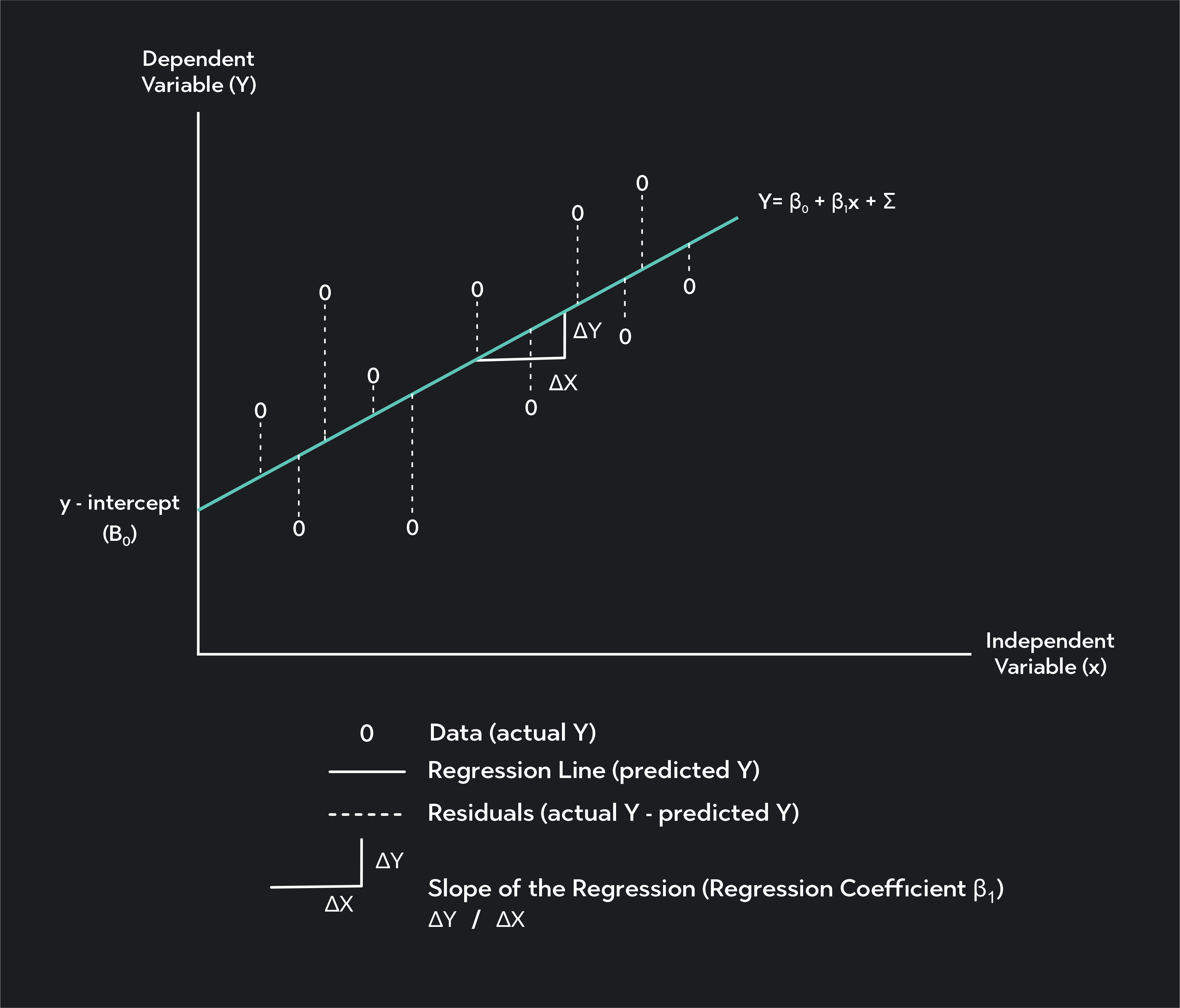
This graph illustrates the key elements of a simple linear regression model. The solid line is the regression line (predicted Y), which is defined by its y-intercept ($\beta_0$) and slope ($\beta_1$). The small circles are the actual data points, and the dotted lines show the residuals (errors), which are the differences between the actual and predicted Y values.

Interpreting the Model's Coefficients

The power of regression lies in the interpretation of its coefficients, $β_{0}$ and $β_{1}$ . These are the parameters that describe the specific linear relationship found in your data.

The Intercept ( $β_{0}$ )

The intercept is the predicted value of the dependent variable (Y) when the independent variable (X) is equal to zero.

The Slope ( $β_{1}$ )

The slope is the most important part of the model. It quantifies the relationship between X and Y. The slope represents the predicted change in Y for a one-unit increase in X.

If $β_{1}$ is positive, Y is predicted to increase as X increases.
If $β_{1}$ is negative, Y is predicted to decrease as X increases.
If $β_{1}$ is zero, there is no linear relationship between X and Y.

7.2: Simple Linear Regression - Statistics LibreTexts

This text from LibreTexts offers very clear examples of how to interpret the slope and intercept in a real-world context.

Read the two paragraphs starting with the interpretation, including the two examples about stream flow and rainfall. Pay close attention to how the verbal interpretation of the slope and intercept is phrased.

A crucial point about the intercept: its interpretation is only meaningful if X=0 is a plausible and relevant value within the context of your data. For example, if your independent variable is a person's weight, the intercept (the predicted blood pressure for a person weighing 0 kg) is biologically meaningless and serves only as a mathematical anchor for the regression line. However, if your independent variable is "number of alcoholic drinks per week," the intercept (the predicted blood pressure for someone who drinks 0 drinks per week) is perfectly meaningful.

The following video provides another excellent walkthrough of interpreting these coefficients.

Regression and R-Squared (2.2)

This video, "Regression and R-Squared (2.2)" from Simple Learning Pro, provides a concise visual explanation of the regression line and how to interpret its slope and intercept.

Watch the first part of the video from the beginning to the end of the GPA example. This will reinforce the meaning of the slope (b_1) and intercept (b_0) and how to use the regression equation for prediction.

Is the Relationship Significant?

In our last lesson, we learned about p-values. In regression, the most important p-value is the one associated with the slope coefficient, $β_{1}$ . It tests the null hypothesis that $β_{1} = 0$ .

Null Hypothesis ( $H_{0}$ ): $β_{1} = 0$ . (There is no linear relationship between X and Y).
Alternative Hypothesis ( $H_{a}$ ): $β_{1} \neq = 0$ . (There is a linear relationship between X and Y).

If the p-value for the slope is less than our significance level (e.g., < 0.05), we reject the null hypothesis and conclude that there is a statistically significant linear relationship between the two variables.

Let's see what this looks like in a typical output from a statistical program like R.

Simple Linear Regression | An Easy Introduction & Examples

The Scribbr article provides a detailed breakdown of a standard regression output table, explaining each column.

Please read the section titled Interpreting the results. Focus on the "Coefficients" table. Understand what the Estimate, Std. Error, t value, and Pr(>|t|) columns represent for both the (Intercept) and the income variable (the slope).

How Well Does the Model Fit? R-squared ( $R^{2}$ )

Knowing the direction and significance of a relationship is important, but we also want to know how strong it is. How well does our line actually fit the data points? This is where R-squared ( $R^{2}$ ), also called the Coefficient of Determination, comes in.

$R^{2}$ is a value between 0 and 1 (or 0% and 100%) that represents the proportion of the variance in the dependent variable (Y) that is explained by the independent variable (X).

An $R^{2}$ of 0 means our model explains none of the variability in Y. The line is no better at predicting Y than simply using the average value of Y.
An $R^{2}$ of 0.60 means that 60% of the variability in Y can be explained by its linear relationship with X. The remaining 40% is due to other factors (the error term, $ϵ$ ).
An $R^{2}$ of 1 means our model explains all the variability. All data points fall perfectly on the regression line.

The following video provides one of the clearest explanations of R-squared available. It intuitively builds the concept from scratch, which will be very helpful.

R-squared, Clearly Explained!!!

This StatQuest video, "R-squared, Clearly Explained!!!", is famous for its exceptionally clear and intuitive explanation of R-squared.

Please watch the entire video (11 minutes). It will walk you through: Why R-squared can be more intuitive than the correlation coefficient, R. The concepts of variation around the mean and variation around the regression line. How R-squared is calculated as the percentage of variation explained by the model. How to interpret different R-squared values in practice.

Putting It All Together: An Example

Let's interpret a full regression output using what we've learned. The image below shows the results of a model predicting a car's fuel efficiency (MPG.city) from its price (Min.Price).

This image shows the R output for a simple linear regression model. It highlights the intercept and slope coefficients and states the final regression equation.

Let's dissect this output:

Coefficients:
- Intercept ( $β_{0}$ ): 26.58. This is the predicted city MPG for a car with a minimum price of $0. As we discussed, this isn't a meaningful real-world scenario, but it's the mathematical starting point for our line.
- Slope ( $β_{1}$ ) for Min.Price: -0.34. This is the key finding. For every one-unit increase in Min.Price (assuming the unit is $1,000), the city MPG is predicted to decrease by 0.34. The negative sign indicates an inverse relationship: more expensive cars tend to have lower fuel efficiency.
Statistical Significance:
- The p-value for Min.Price is 2.64e-07, which is a tiny number ( $0.000000264$ ). Since this is far less than 0.05, we can confidently reject the null hypothesis and conclude that there is a highly statistically significant negative relationship between price and city MPG.
Model Fit (R-squared):
- The Multiple R-squared is 0.4412. This tells us that 44.12% of the variation in city MPG among these cars can be explained by their minimum price. While this is a significant relationship, it also means that about 56% of the variation is due to other factors not included in this simple model, such as engine size, vehicle weight, or transmission type.

The final equation, $y^= 26.58 - 0.34 x$ , summarizes this entire model.

Conclusion

In this lesson, you've learned how to interpret the results of a simple linear regression, one of the most common statistical models in science.

Here are the key takeaways:

Simple linear regression models the relationship between two quantitative variables using a straight line: $Y = β_{0} + β_{1} X + ϵ$ .
The intercept ( $β_{0}$ ) is the predicted value of Y when X is 0, which may or may not be practically meaningful.
The slope ( $β_{1}$ ) is the core of the model: it tells you the predicted change in Y for every one-unit increase in X.
The p-value for the slope tests whether the linear relationship is statistically significant.
R-squared ( $R^{2}$ ) measures model fit by quantifying the percentage of variation in the dependent variable that is explained by the independent variable.

So far, we have discussed modeling a continuous outcome (like blood pressure or MPG). But in epidemiology, we are often interested in binary outcomes: getting a disease versus not getting it, surviving versus not surviving. A straight line doesn't work for that. In our next lesson, we will tackle this challenge by introducing logistic regression, a powerful technique for modeling "yes/no" outcomes.

Recommended resources