Understanding Time-Dependent Covariates

What is a Time-Dependent Covariate?

Up to this point, all the covariates we've considered in our models—like sex, age at diagnosis, or baseline disease stage—have been time-fixed. Their values are measured once at the beginning of the study and are assumed to remain constant throughout the follow-up period.

However, in reality, many important characteristics are dynamic. A patient's health status, treatments, and exposures can change over time. A time-dependent covariate (also called a time-varying covariate, or TVC) is simply a variable whose value is not fixed but can change during follow-up.

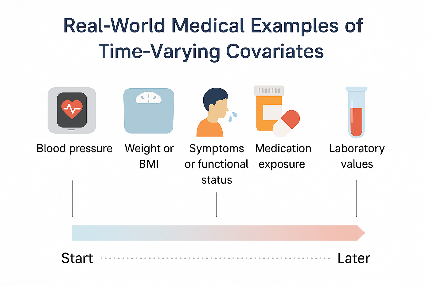
At first, this might seem to contradict the "proportional hazards" assumption of the Cox model. If a covariate's value is changing, how can the hazard ratio associated with it be constant? The following reading explains the elegant theoretical solution to this apparent paradox.

Let's summarize the two key ideas from the reading:

1. Instantaneous Proportionality: The Cox model's proportional hazards assumption holds at any given instant in time. The model's formula is written as:

   $$h_i(t)=h_0(t)\exp ({\beta }^{\prime }{X}_i(t))$$

   The crucial part is $X_i(t)$—the covariate vector for person $i$ is now a function of time $t$. This means the model compares individuals based on their covariate values at the exact moment an event occurs, not just their baseline values.

2. The start-stop Data Format: To handle this in practice, we restructure the data. Instead of one row per patient, a patient's follow-up is sliced into multiple rows or intervals. A new interval begins whenever a time-dependent covariate changes its value. Within each interval, the covariate is constant. This format, also known as the counting process format, allows the software to know the precise value of all covariates for every person at risk at every event time.

The following short video clip visually explains this practical data restructuring.

When are TDCs Necessary? The Problem of Immortal Time Bias

Now we know what TDCs are. But why are they so important? They are necessary whenever a key exposure or predictor can change during follow-up. Failing to account for this change doesn't just reduce a model's accuracy; it can introduce a severe and misleading form of bias.

The most famous example of this is immortal time bias. This bias occurs when a study group is defined by an event that happens after follow-up begins. To be in that group, a person must survive the period between the start of the study and the event. This period of guaranteed survival is called "immortal time."

Let's make this concrete with the classic Stanford heart transplant study. In this study, patients were enrolled when they were placed on a waitlist for a transplant. Some received a transplant, others did not. A naive analysis might compare the "transplanted" group to the "non-transplanted" group from day one.

The following video brilliantly demonstrates the flaw in this approach.

The video's numerical example is the heart of the matter.

• Incorrect (Biased) Method: All follow-up time for a patient who eventually gets a transplant is counted in the "transplant" group, right from day zero. This includes the "immortal" waiting period before the surgery, during which they could not have died and still received a transplant. This artificially lowers the death rate in the transplant group.
• Correct (Time-Varying) Method: A patient's follow-up time is split. The time before their transplant is correctly attributed to the "non-transplant" group. Only the time after the transplant is attributed to the "transplant" group. The patient effectively moves from one group to the other at the time of surgery.

This next image provides a perfect visual summary of the problem and its solution.

As you can see, the time-varying analysis (Panel C) is the only method that correctly attributes person-time. This is precisely what we achieve by modeling treatment as a time-dependent covariate.

Immortal time bias is not a niche academic issue. As the video mentions, it has been found in numerous published studies, often leading to wildly optimistic conclusions about the effectiveness of treatments. It is a critical flaw to look for when evaluating any observational study where the exposure of interest can begin after follow-up starts.

Internal vs. External Covariates: An Important Distinction

Finally, it's useful to distinguish between two types of TDCs, because the distinction has important implications for how we interpret our model.

As the article explains:

• External (or Exogenous) TDCs: These are variables whose values are not influenced by the individual patient's journey. Examples include things like daily air pollution levels or seasonal changes. Their paths are determined by outside forces.
• Internal (or Endogenous) TDCs: These are processes generated by the individual, and they require the person to be alive to be measured. Examples include biomarkers (like blood pressure), symptom severity, or the initiation of a new treatment based on the patient's condition.

While the Cox model can handle both types mechanically, interpreting the results for internal covariates requires great care. When an internal covariate (like a worsening lab value) influences a doctor's decision to start a treatment (another internal TDC), you can get a feedback loop known as time-dependent confounding. In this situation, the model coefficient for the treatment measures its association with the outcome conditional on the lab value, which may not be the same as the overall causal effect of the treatment. Untangling this is a complex topic for advanced causal inference, but being aware of this distinction between association and causation is a key step in sophisticated interpretation.

Conclusion

In this lesson, we have moved beyond fixed, baseline characteristics to the dynamic world of time-dependent covariates. This is a crucial step for accurately modeling real-world health processes.

Here are the key takeaways:

• A time-dependent covariate (TDC) is a variable whose value can change over the course of a study's follow-up period.
• TDCs are necessary whenever a key predictor is not constant, such as when a treatment is initiated after follow-up begins.
• Failing to model a time-dependent exposure correctly can lead to immortal time bias, which creates a spurious survival advantage for the exposed group by misattributing a period of guaranteed survival.
• The correct approach involves a time-varying analysis, where a subject's exposure status changes at the time the event occurs. This is achieved by restructuring the data into a start-stop format.
• It is important to distinguish between external (e.g., pollution) and internal (e.g., biomarkers, treatments) TDCs, as internal covariates can introduce complex interpretive challenges like time-dependent confounding.

You now understand the critical importance of identifying and correctly conceptualizing time-dependent covariates to avoid major analytical errors. In our next lesson, we will build directly on this foundation and learn how to interpret the output of a Cox model that includes a time-dependent covariate.