Stratified Cox Models: Purpose and Interpretation

When Proportionality Fails: The Need for Stratification

Let's begin by recapping the core issue. The standard Cox model, with its formula $h(t)=h_0(t)\exp ({\beta }_1{X}_1+\cdots +{\beta }_p{X}_p)$, rests on the assumption that all individuals in the study share a single, common baseline hazard function, $h_0(t)$. A covariate that violates the PH assumption is one where the hazard ratio is not constant over time. This effectively means that the shape of the hazard function is different for different levels of that covariate, which contradicts the "single baseline hazard" assumption.

So, how can we fix this? Instead of forcing all groups to share the same baseline hazard, what if we allowed certain groups to have their own? This is precisely the logic of stratification.

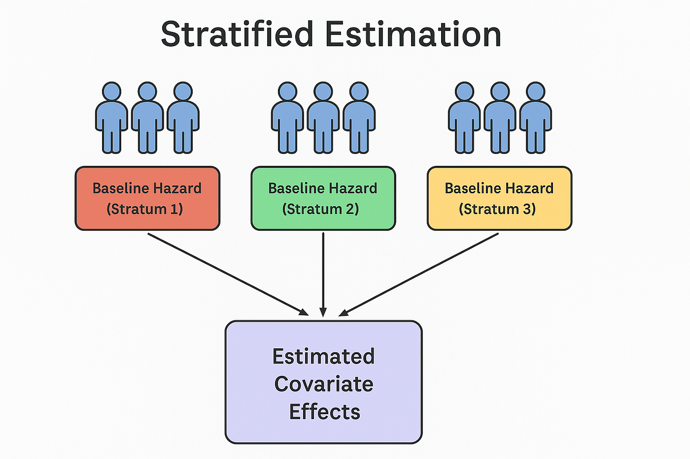
The stratified Cox model divides the study population into distinct groups, or strata, based on the levels of the problematic covariate. It then estimates a separate baseline hazard function for each stratum. The key, however, is that it still estimates a single, common set of coefficients ($\beta$) for the other covariates across all strata.

This diagram provides a great conceptual overview of the process.

To formalize this idea, let's look at the underlying mechanics.

The formula from the reading is the most important part to understand:

Let's break this down:

• ${\lambda }_{ij}(t)$ is the hazard for the $i$-th person, who belongs to stratum $j$.
• ${\lambda }_{0j}(t)$ is the baseline hazard for stratum $j$. The subscript $j$ is the crucial modification. It signifies that each stratum gets its own unique baseline hazard function. This is how the model accommodates the non-proportionality.
• $\exp (x_i^T\beta )$ represents the effect of the other covariates. Notice that the coefficient vector $\beta$ does not have a subscript $j$. This means the hazard ratios for these covariates are assumed to be the same across all strata.

In essence, we are letting the baseline risk vary freely between, for example, males and females (by stratifying on sex), while still estimating a single, unified effect of a new drug treatment across both groups.

Interpreting the Output of a Stratified Cox Model

Now that you understand the "why," let's move to the "how." How do you interpret the results once you've fit a stratified model? The most important thing to realize is that the variable you stratify on is treated differently from the other covariates.

Because the model estimates a separate baseline hazard for each stratum instead of a single coefficient, the stratification variable is removed from the main coefficient table. You will not get a hazard ratio or a p-value for it. This is by design. Its effect is absorbed into the differing shapes of the baseline hazard functions.

The following reading provides an excellent walkthrough. Although the code examples are in Python, the model output and interpretation principles are universal and apply directly to R as well.

As the article demonstrates, the interpretation of the other covariates in the model is exactly the same as in a standard Cox model. For a given covariate:

• The coefficient ($\beta$) is the log-hazard ratio.
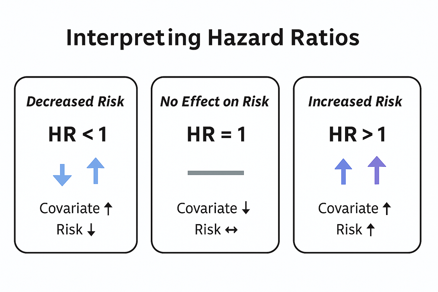
• The hazard ratio ($e^{\beta }$) is the multiplicative change in hazard for a one-unit increase in the covariate, holding all other covariates constant and within any given stratum.
• The p-value and confidence interval are interpreted in the usual way to assess statistical significance.

This diagram serves as a quick reminder for interpreting any hazard ratio you encounter in the model's output.

The process, therefore, is:

1. Identify which variable(s) were used for stratification.
2. Acknowledge that you cannot make a direct inferential statement (i.e., get a single HR or p-value) about their effect from the model summary.
3. Interpret the HRs for all other covariates in the model as you normally would.

Limitations and Final Considerations

While stratification is an elegant solution, it's not without trade-offs. It's crucial to understand its limitations to know when it's the right tool for the job.

Let's summarize the main drawbacks:

• You lose the ability to estimate the effect of the stratification variable. This is the most significant limitation. If the variable violating the PH assumption is the main exposure or treatment you want to study, stratification is a poor choice because it prevents you from getting the very hazard ratio you are interested in. It's best used for "nuisance" confounders that you need to control for but aren't the focus of your analysis.
• It is best suited for categorical variables. While you can stratify on a continuous variable by cutting it into categories (e.g., age <50, 50-70, >70), the choice of cut-points can be arbitrary and can lead to a loss of information.
• There can be a minor loss of statistical power. By estimating multiple baseline hazard functions instead of just one, the model is more flexible but slightly less efficient. This might result in slightly wider confidence intervals for the other covariates compared to a standard Cox model (if the PH assumption had held).

Conclusion

In this lesson, we've added an essential technique to your survival analysis toolkit. When faced with a categorical covariate that violates the proportional hazards assumption, you now have a robust method for handling it.

Here are the key takeaways:

• The stratified Cox model is used to adjust for a covariate that violates the proportional hazards assumption.
• It works by estimating a separate and unique baseline hazard function for each level (stratum) of the problematic variable.
• The hazard ratios for all other covariates in the model are assumed to be constant across the strata.
• When interpreting the output, the stratification variable will not appear in the coefficient table and will not have a hazard ratio. The coefficients for the remaining variables are interpreted just as they would be in a standard Cox model.
• This method is ideal for controlling for non-proportional "nuisance" variables, but not for your primary variable of interest.

You are now equipped to handle one of the most common challenges in Cox regression. However, as we've discussed, stratification isn't always the right answer, especially when the main exposure variable itself has non-proportional hazards.

In our next lesson, we will address that exact scenario by exploring another advanced technique: modeling with time-dependent covariates. This approach will allow us to explicitly estimate how a hazard ratio changes over time, providing an even deeper insight into the dynamics of risk.