Welcome to our next session. In the previous lesson, we established the theoretical foundation of the Cox proportional hazards model, focusing on its single most important rule: the proportional hazards (PH) assumption. We learned that this assumption dictates that the hazard ratio between any two groups must remain constant over time.
This lesson moves from theory to practice. Knowing the rule is one thing; verifying that it holds true for your specific data is another. Today, you will learn how to use graphical methods to assess whether the proportional hazards assumption is met. We will primarily focus on a technique called the log-log survival plot, which is a standard diagnostic tool in survival analysis. This is a critical step in validating your Cox model and ensuring your conclusions are reliable.
The Logic of Graphical Checks
Before diving into the specific method, let's consider why a graphical check is so useful. The PH assumption implies a very specific mathematical relationship between the survival curves of different groups. While the raw Kaplan-Meier survival curves can give us a hint—as we saw, crossing curves are a major red flag—they don't tell the whole story.
We need a tool that transforms the data in a way that makes violations of the assumption visually obvious. The log-log plot does exactly this.
Log-Log Survival Plots: The Primary Tool
The core idea behind a log-log plot is to apply a mathematical transformation to the estimated survival function, . Specifically, we plot against the logarithm of time. While the formula might seem opaque, the intuition behind it is straightforward. This particular transformation has a special property: if the proportional hazards assumption holds true for a categorical covariate, the transformed survival curves for each category should be approximately parallel.
Let's explore the reasoning behind this. The following article by Kelvin Foo provides a clear explanation.
Survival Analysis and Cox Proportional Hazards Model | by Kelvin Foo
This article section explains how the Cox model's survival function can be transformed to check the PH assumption.
Please read the section titled "Evaluating Cox PH Assumptions," focusing on the first part, "Graphical Approach 1: Log-Log Plots". You don't need to derive the equations yourself, but focus on the final conclusion: the transformation is designed so that the difference between the curves for two groups becomes a constant that does not involve time, resulting in parallel lines.
The key takeaway is that the log-log transformation converts the multiplicative relationship of hazards into an additive one. The vertical distance between two parallel log-log curves is related to the log of the hazard ratio. If this distance remains constant across time (i.e., the lines are parallel), it implies the hazard ratio is also constant.
The following short video clip from the TileStats channel reinforces this exact point.
The Cox proportional hazards model explained
This video provides a quick verbal and visual summary of using log-log plots.
Watch the brief segment from this explanation about checking the assumption. Note the clear rule: "to fulfill the proportional hazards assumption the curves should be approximately parallel."
Interpreting a Real Log-Log Plot
Now, let's apply this to an example. The plot below was generated to check the PH assumption for the IsBorrowerHomeowner variable in a financial dataset, where the event is likely loan default.
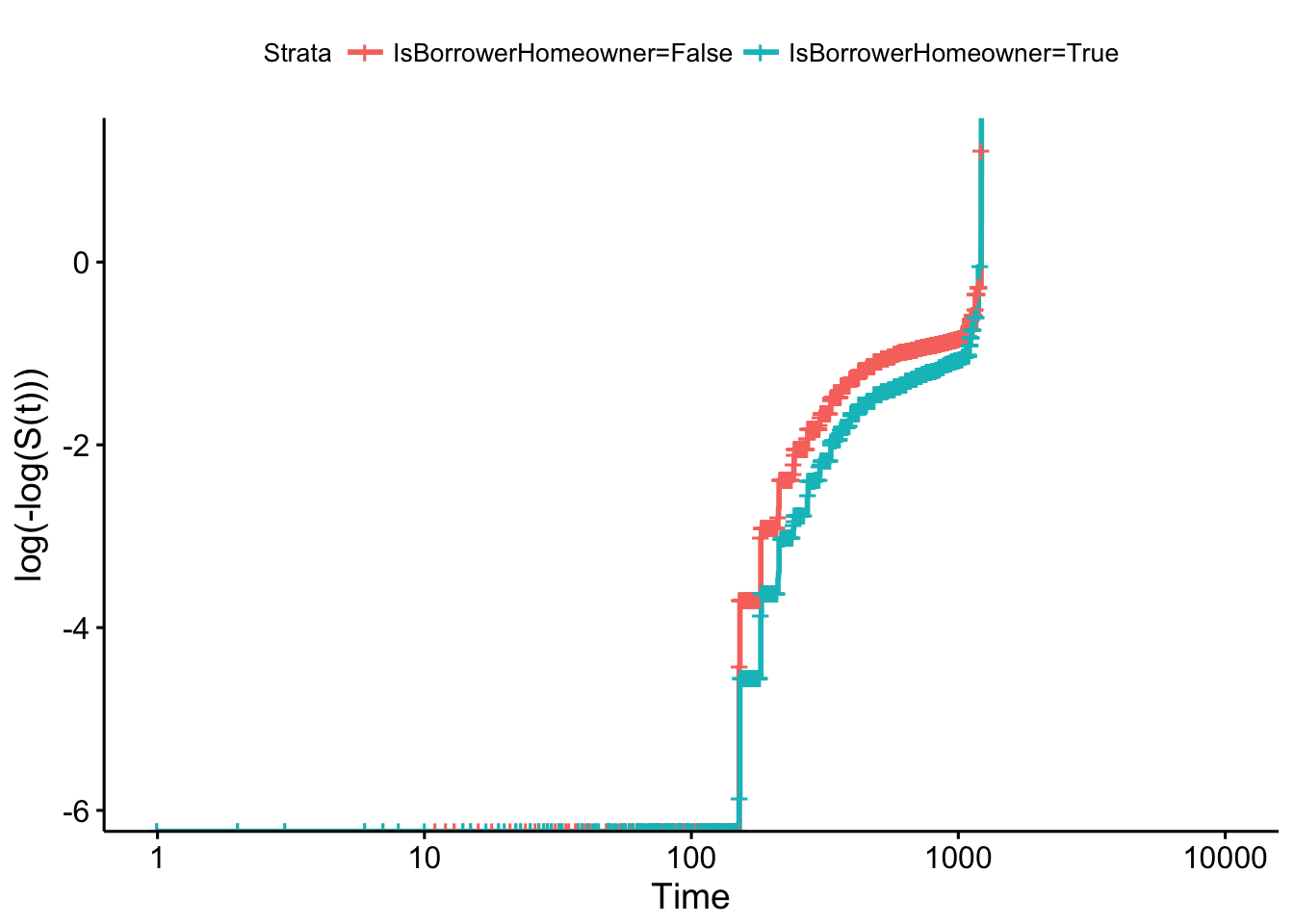
How do we interpret this? We look at the two curves and visually assess if they are parallel. In this plot, the red and teal curves track each other quite closely. Although they are not perfectly parallel (real-world data is rarely perfect), there is no strong evidence of them converging or diverging systematically. Therefore, based on this graphical check, we would conclude that the proportional hazards assumption is reasonably satisfied for the IsBorrowerHomeowner variable.
It is important to acknowledge that this method has a degree of subjectivity. The resource from which this plot was taken makes this exact point.
3.6 How to evaluate the PH assumption?
This chapter excerpt from a survival analysis course provides more context on the log-log plot method.
Please read the section titled "Graphical approach". Pay special attention to the practical issue raised: "how to decide 'how parallel is parallel?'".
As the text suggests, the decision can be subjective. The general advice is to be conservative: unless the lines show a clear and systematic trend of non-parallelism (e.g., they cross or are rapidly moving apart), you can often proceed with the assumption that the PH condition is met.
An Alternative Graphical Check: Observed vs. Expected Curves
Another intuitive graphical method involves comparing the observed survival curve with the one predicted by your fitted Cox model. The logic is as follows:
- Observed Curve: For each level of a categorical predictor (e.g., "male" and "female"), you generate a Kaplan-Meier survival curve directly from the data. This is a non-parametric estimate of what actually happened in your sample.
- Expected Curve: You use your fitted Cox model to predict the survival curve for each of those same levels. This is what the model thinks the survival curve should look like.
- Compare: You plot the observed and expected curves for each group on the same graph.
If the observed and expected curves for a group are very close, it means the model is a good fit for that group, and the PH assumption likely holds. If the curves diverge substantially, it suggests the model's single hazard ratio is not adequately describing the relationship over time.
The article by Kelvin Foo that you read earlier also describes this method.
Survival Analysis and Cox Proportional Hazards Model | by Kelvin Foo
This section briefly explains the observed vs. expected plot method.
Now, please read the short section titled "Graphical Approach 2: Observed vs Expected Plots".
This method is conceptually straightforward and provides another way to visually diagnose potential problems with the PH assumption.
Conclusion
In this lesson, we transitioned from understanding what the proportional hazards assumption is to actively checking it with data. These graphical checks are a fundamental part of responsible survival modeling.
Here are the key takeaways:
- Graphical methods provide an intuitive way to assess the proportional hazards assumption.
- The primary method is the log-log survival plot, which plots
log(-log(S(t)))against log(time). - The rule for interpreting a log-log plot is simple: if the curves for different groups are approximately parallel, the PH assumption is likely met. If they cross or systematically diverge, the assumption is violated.
- An alternative method is to compare observed (Kaplan-Meier) survival curves with expected (Cox model-predicted) curves. A close match supports the PH assumption.
- A key limitation of graphical checks is their subjectivity. Deciding what counts as "parallel enough" can be ambiguous.
This final point leads us directly to our next topic. While graphs are excellent for building intuition, we often need a more objective, quantitative measure to confirm our suspicions. In the next lesson, we will explore a formal statistical test for the PH assumption based on an analysis of Schoenfeld residuals. This will provide us with a p-value to help make a more definitive judgment on the validity of our Cox model.