Proportional Hazards Assumption

The Core Principle: A Constant Hazard Ratio

At its heart, the Cox proportional hazards model gets its name directly from its core assumption.

As the reading states, the proportional hazards (PH) assumption is that the hazard ratio between any two groups remains constant over time. The absolute risk for everyone in the study might increase or decrease as time goes on, but the relative risk (the hazard ratio) between a treated patient and a control patient, or between a male and a female patient, is assumed to be stable throughout the entire follow-up period.

The GraphPad guide offers another excellent phrasing of this same principle.

This idea of a "scaled version" is key. The Cox model doesn't make any assumptions about the shape of the baseline hazard function, $h_0(t)$—it can be a complex, wiggly line. This is the "non-parametric" part of the model. However, it assumes that the hazard function for any individual with a specific set of covariates (e.g., male, age 50, on treatment) is simply that baseline hazard function multiplied by a constant factor:

Notice that the time variable, $t$, only appears in the baseline hazard $h_0(t)$. The part that depends on the covariates, $\exp (\dots )$, is constant with respect to time. This mathematical structure is the formal expression of the proportional hazards assumption.

An Analogy to Other Regression Models

For someone with your background in information systems and interest in machine learning, it can be helpful to draw parallels to other regression models you may have encountered. The idea of a constant effect is not unique to Cox regression.

The following video does an excellent job of building this intuition by relating proportional hazards to the assumptions of linear and logistic regression.

Let's summarize the analogy presented in the video:

• Linear Regression: In a simple model without interaction terms, we assume the difference in the mean outcome between two groups is constant. For example, the difference in average salary between two departments is the same regardless of an employee's years of experience.
• Logistic Regression: Similarly, we assume the odds ratio is constant. The odds of a customer churning if they are on "Plan A" versus "Plan B" is the same, regardless of their age.
• Cox Regression: The equivalent assumption is that the hazard ratio is constant over time. If a new drug cuts the hazard of death in half (HR = 0.5) compared to a placebo, the PH assumption means it cuts the hazard in half on Day 1, Day 100, and Day 500. The relative benefit doesn't change over time.

Visualizing Proportional vs. Non-Proportional Hazards

Visualizing what this means for the hazard functions can make the concept much clearer.

When hazards are proportional, their curves on a regular scale will move up and down together, maintaining a constant ratio. If you plot the logarithm of the hazard, the curves will be parallel—separated by a constant vertical distance. This constant distance is the log of the hazard ratio.

What does a violation look like? A violation means the effect of a covariate changes over time.

• Example 1: A surgery might dramatically reduce the hazard of death in the short term, but its benefit diminishes over years. The hazard ratio would be low initially but would approach 1.0 as time passes.
• Example 2: One treatment might be riskier at the beginning but offer better long-term survival than another.

A classic sign of non-proportional hazards is when the Kaplan-Meier survival curves for two groups cross.

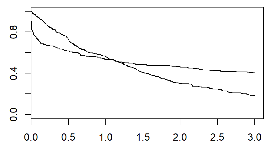
The TileStats channel provides a brief but clear verbalization of why this is a problem.

If the survival curves cross, one group has a higher risk of the event for part of the study, and the other group has a higher risk for another part. A single, constant hazard ratio cannot possibly describe this changing relationship. The assumption is violated.

Other Assumptions of the Cox Model

While the proportional hazards assumption is the most defining one, it's not the only one. For context, it's useful to be aware of the others, though we won't detail them today. The GraphPad checklist you viewed earlier also lists these. The main ones include:

• Non-informative censoring: The reason a subject is censored (e.g., moved away, study ended) is not related to their prognosis.
• Independence of survival times: The survival time of one subject is independent of another's. This is a standard assumption in most regression models.
• Linearity for continuous variables: The effect of a continuous predictor is assumed to be linear on the log-hazard scale.

For today, the crucial focus remains squarely on understanding proportionality.

Conclusion

In this lesson, we have defined and explored the single most important assumption of the Cox model. Your interpretations of hazard ratios from the previous lesson are only meaningful if this assumption holds true.

Here are the key takeaways:

• The proportional hazards (PH) assumption states that the effect of any covariate on the hazard is constant over time.
• This means the hazard ratio comparing any two individuals or groups is stable throughout the entire follow-up period.
• Visually, this implies that the log-hazard curves for different groups are parallel, and their survival curves should not cross.
• A violation occurs when the effect of a variable changes over time, such as a treatment effect that wanes or a risk factor that only becomes relevant late in the process.

Now that we know what the proportional hazards assumption is and why it's so important, a critical question arises: how do we check if it's true for our data? In our next lesson, we will begin to answer that by exploring graphical methods used to assess the PH assumption.