Interpreting Cox Models with Time-Dependent Covariates

Interpreting the Effect of a Time-Dependent Covariate

Let's start by recalling what a time-dependent covariate is. It is any predictor variable whose value can change during the study's follow-up period.

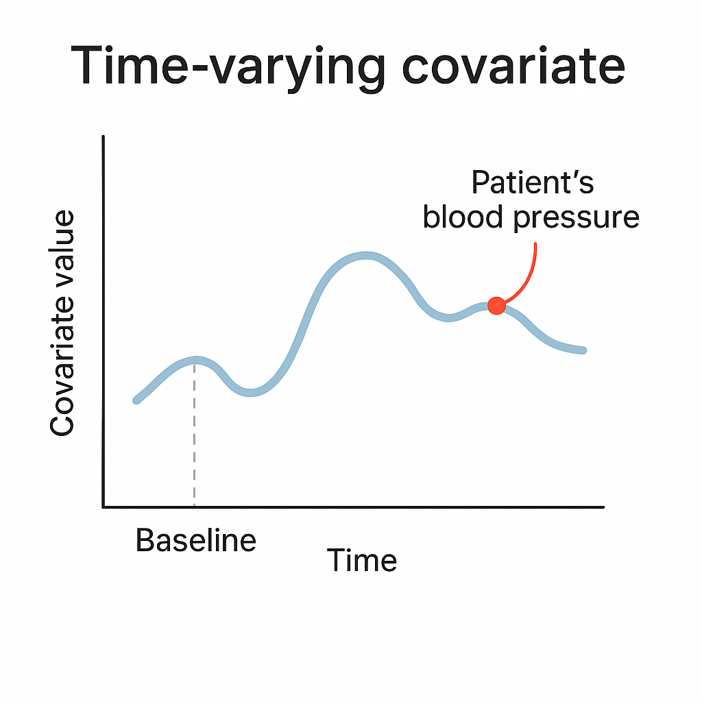
When we include such a variable in a Cox model, its coefficient tells us about the instantaneous risk associated with its value at any given moment in time. To see this in practice, we will use a fantastic and comprehensive guide on Cox regression in R. We will be referring to the Rossi dataset mentioned in this document, which tracks recidivism (rearrest) among 432 individuals after release from prison.

First, let's look at the output for a model with a time-dependent covariate and see how to interpret it.

Let's break down the key part of that output for mod.allison.2:

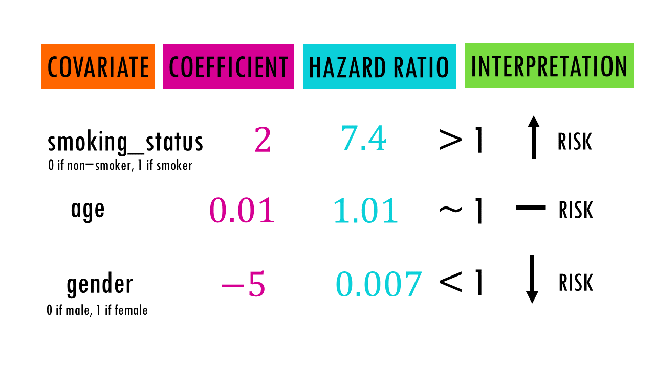
The interpretation follows the same logic as for any other variable in a Cox model, but with a specific time-dependent framing.

• The Coefficient (coef): The value -1.3283 is the estimated log-hazard. A negative value suggests a protective effect.
• The Hazard Ratio (exp(coef)): This is the most interpretable value. Here, it is $e^{-1.3283}\approx 0.265$.
• The Interpretation: We say that at any given point in time, the hazard of rearrest for an individual who is employed is only 0.265 times the hazard for an individual who is not employed, holding all other covariates constant. Put another way, being employed is associated with a $(1-0.265)\times 100\%=73.5\%$ reduction in the instantaneous risk of rearrest.

This interpretation is powerful because it correctly reflects the changing nature of employment status.

Case Study: Interpreting the Fix for Immortal Time Bias

In the last lesson, we discussed how a naive analysis of the Stanford Heart Transplant data could lead to immortal time bias. Now, let's look at the actual output to see how using a time-dependent covariate corrects this.

Let's compare the results side-by-side:

1. Naive (Biased) Model:

   • Coefficient (TSTAT): -1.999
   • Hazard Ratio (Risk Ratio): 0.135
   • Biased Interpretation: This model suggests that receiving a heart transplant reduces the hazard of death by about 86.5%. As we know, this result is artificially inflated by immortal time bias.

2. Correct (Time-Dependent) Model:

   • Coefficient (TSTAT): -0.966
   • Hazard Ratio (Risk Ratio): 0.381
   • Correct Interpretation: At any given point in time, the hazard of death for a patient who has received a transplant is 0.381 times the hazard for a patient who is still waiting for one. This translates to a 61.9% reduction in instantaneous risk.

The difference is stark. The correct model still shows a substantial benefit from transplantation, but the effect is much smaller than the biased estimate suggested. This comparison powerfully illustrates how crucial the correct analytical approach—and its interpretation—is to arriving at a valid conclusion.

An Interpretive Wrinkle: Lagged Covariates and Causality

Your background in information systems might lead you to think about the direction of causality. In the recidivism example, does being employed prevent arrest, or does being arrested prevent employment? The latter is certainly true! This is a classic problem of reverse causation.

One common, though imperfect, way to address this is to use a lagged value of the covariate. Instead of using employment status in the current week to predict arrest in that same week, we can use employment status from the previous week.

Let's return to the LINK PDF to see how this changes the interpretation.

In the lagged model (mod.allison.3), the coefficient for the lagged employed variable is -0.7869, which gives a hazard ratio of $e^{-0.7869}\approx 0.455$.

The interpretation is now: "Being employed in the previous week is associated with a 54.5% reduction in the hazard of rearrest in the current week."

Notice that the effect is smaller than the 73.5% reduction we saw in the non-lagged model. This is very common. The lagged analysis provides a more conservative and often more plausible estimate of the effect by slightly disentangling the immediate feedback loop between employment and arrest.

Using TDCs to Test the Proportional Hazards Assumption

Finally, one of the most important uses of time-dependent covariates is to formally test the proportional hazards (PH) assumption itself. If the effect of a covariate changes over time, then the hazards are not proportional. We can model this by creating a special kind of TDC: an interaction term between the covariate and a function of time.

In model mod.allison.5, the output for the interaction term age:stop is:

Here, the interpretation is different. We are not interested in the hazard ratio itself. Instead, we look at the p-value.

• The small p-value (0.009) indicates that the interaction term is statistically significant. This provides evidence against the proportional hazards assumption for the variable age. It tells us the effect of age is not constant over time.
• The negative coefficient (-0.0038) tells us the direction of this change. It means that the effect of age (its log-hazard) becomes more negative, or less positive, as time goes on. In this context, the impact of a person's age on their risk of rearrest diminishes over the follow-up period.

This is a powerful diagnostic tool that is made possible by the framework of time-dependent covariates.

Conclusion

In this lesson, we moved from theory to practice, learning how to interpret the output of a Cox model with time-dependent covariates. This skill is vital for understanding sophisticated survival analyses and for critically evaluating research findings.

Here are the key takeaways:

• The hazard ratio for a TDC represents the instantaneous risk ratio. It compares individuals based on their covariate status at a specific moment in time.
• Using TDCs is the correct way to analyze exposures that begin after follow-up starts, and interpreting the output correctly reveals an unbiased effect estimate, as seen in the heart transplant example.
• Thinking about causality is important. Using lagged covariates is one way to create a more conservative and plausible estimate when reverse causation is a concern.
• TDCs can be used as a diagnostic tool. A significant interaction between a covariate and time is evidence that the proportional hazards assumption does not hold for that covariate.

We have now covered how to handle covariates that don't have proportional hazards, either through stratification or by modeling them as time-dependent. In our next lesson, we will turn our attention from the covariates to the outcome, exploring the challenge of competing risks, which arise when individuals can experience more than one type of event.