Competing Risks Modeling with `cmprsk` in R

What are Competing Risks and Why Do They Matter?

Before diving into the R code, let's quickly recap the core concepts. In a competing risks scenario, simply treating the "other" events as censored is incorrect. Censoring assumes that if we could follow the subject long enough, they might still experience the event of interest. However, if a patient dies of a heart attack (a competing event), they are no longer at risk of dying from cancer (the primary event). This violates the core assumption of non-informative censoring.

Using a standard Kaplan-Meier curve to estimate the probability of one event type will lead to an overestimation of the true incidence.

The following video provides an excellent summary of these foundational concepts.

As the video explains, we need two specialized tools to handle competing risks:

1. Cumulative Incidence Function (CIF): This estimates the probability of a specific event occurring by time t, accounting for the fact that other competing events could happen first. It is the correct non-parametric alternative to the (1 - Kaplan-Meier) estimator.
2. Competing Risks Regression Models: These models allow us to assess how covariates influence the risk of specific events. There are two primary types:
   • Cause-Specific Hazard Models: Focus on the instantaneous rate of an event in subjects who are still event-free. Best for etiological questions (e.g., "Does this gene increase the rate of cancer-related death among those still alive?").
   • Subdistribution Hazard (Fine-Gray) Models: Focus on the effect of a covariate on the cumulative incidence itself. Best for prognostic questions (e.g., "Does this treatment reduce a patient's overall probability of dying from cancer over five years?").

Given your interests in data science and prediction, the Fine-Gray model is particularly relevant as its output directly relates to the probability of an outcome. We will focus on this model.

Getting Started: Cumulative Incidence Functions in R

Let's begin by analyzing competing risks data non-parametrically. We'll use the Melanoma dataset from the {MASS} package, which is a classic dataset for this topic. A great tutorial by Emily Zabor will guide our practical work.

Let's follow the steps outlined in the reading. First, ensure you have the necessary packages installed and loaded. The {tidycmprsk} package provides a user-friendly interface to the functions in {cmprsk}.

# install.packages(c("MASS", "tidycmprsk", "ggsurvfit", "gtsummary"))
library(MASS)
library(dplyr) # For the mutate function
library(tidycmprsk)
library(ggsurvfit)

As described in the reading, the status variable in the Melanoma dataset needs to be recoded for clarity and for use with the {tidycmprsk} package.

• status = 1: Died from melanoma (our primary event)
• status = 2: Alive (censored)
• status = 3: Died from other causes (the competing event)

The package expects 0 for censored, so we'll recode 2 to 0, and keep 1 as is. For clarity, we'll recode 3 to 2 to represent the second event type.

# Load and prepare the data
data(Melanoma, package = "MASS")

melanoma_data <- Melanoma %>%
  mutate(



    # Recode status: 0=censored, 1=died from melanoma, 2=died from other causes
    status = as.factor(recode(status, `2` = 0, `1` = 1, `3` = 2))
  )




# Check the first few rows
head(melanoma_data)

Now we can calculate and plot the CIFs for both event types (death from melanoma and death from other causes). The cuminc() function does the calculation, and ggcuminc() creates the plot.

# Calculate cumulative incidence
cif_fit <- cuminc(Surv(time, status) ~ 1, data = melanoma_data)




# Plot the CIFs for both event types
ggcuminc(cif_fit, outcome = c("1", "2")) +
  labs(
    x = "Days Since Operation",
    y = "Cumulative Incidence (Probability of Event)"
  ) +
  scale_ggsurvfit() # Use a nice theme and labels

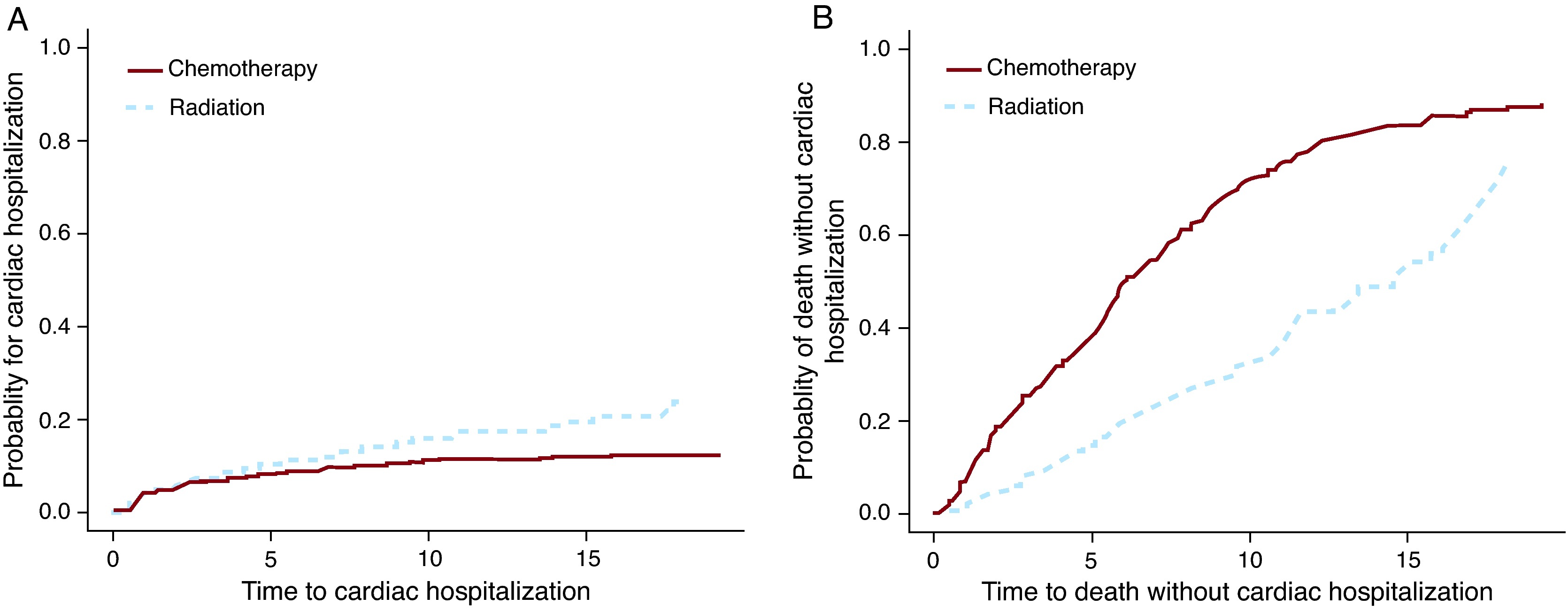
This will produce a plot showing the probability of each event over time. Unlike biased Kaplan-Meier curves, the sum of these probabilities at any given time point represents the total probability of having any event, which can never exceed 100%.

Fine-Gray Competing Risks Regression

Now for the main event: fitting a regression model to understand how covariates affect the incidence of an event. We will fit a Fine-Gray subdistribution hazard model.

The video below explains the theory behind the two main regression models and demonstrates how to interpret their results.

As the video explains, the Fine-Gray model's power is that its coefficients (and their exponentiated form, the subdistribution hazard ratio or SHR) have a direct interpretation on the CIF. An SHR > 1 means the covariate increases the cumulative incidence of the event.

We will use the crr() function from {tidycmprsk} to fit the model. Let's model the effect of tumor thickness and ulcer presence on the incidence of death from melanoma.

Let's apply this to our data. We are interested in status = 1 (death from melanoma) as our event of interest. The competing event is status = 2 (death from other causes). status = 0 is censoring.

# Load gtsummary for beautiful tables
library(gtsummary)




# Fit the Fine-Gray model for death from melanoma (status = 1)
# The `crr` function handles the censoring code (0) and competing events automatically.
crr_fit <- crr(Surv(time, status) ~ thickness + ulcer, data = melanoma_data, failcode = 1)




# Display the results in a formatted table
tbl_regression(crr_fit, exp = TRUE)

The tbl_regression output will look something like this:

Interpreting the Output:

Let's assume your model for melanoma_data produced an SHR of 1.20 for thickness and 2.50 for ulcer (with ulcer=1 for presence).

• Tumor Thickness: The SHR of 1.20 means that for every 1 mm increase in tumor thickness, the subdistribution hazard of dying from melanoma increases by 20%. More importantly, this tells us that thicker tumors are associated with a higher cumulative incidence of death from melanoma.
• Ulceration: The SHR of 2.50 means that the subdistribution hazard of melanoma death is 150% higher for patients with ulceration compared to those without. This indicates that the presence of an ulcer is a strong prognostic factor for a higher probability of dying from melanoma over time.

This interpretation is direct and powerful for making predictions and understanding patient prognosis, which is often the goal in data science and clinical applications.

Conclusion

Congratulations! You have now learned how to handle one of the most common complexities in real-world survival data. By moving beyond standard Cox models, you can produce more accurate and meaningful results when competing events are present.

Here are the key takeaways from this lesson:

• Competing risks occur when an event (e.g., death from other causes) prevents the primary event of interest from happening.
• Standard methods like Kaplan-Meier curves and Cox models are biased in this setting.
• The Cumulative Incidence Function (CIF) is the correct non-parametric method to estimate event probabilities. In R, use cuminc() from the {tidycmprsk} package.
• The Fine-Gray subdistribution hazard model is used for regression when the goal is prognosis. It models the effect of covariates directly on the cumulative incidence. In R, use crr() from {tidycmprsk}.
• The subdistribution hazard ratio (SHR) from a Fine-Gray model tells you about a covariate's effect on the probability (incidence) of an event over time.

This lesson concludes our tour of new analytical methods. In our final lesson, you will get a chance to synthesize everything you've learned—from basic descriptive statistics to Kaplan-Meier curves, Cox models, and competing risks—to conduct a complete survival analysis on a new dataset from start to finish.