End-to-End Data Analysis Techniques

The Project: Survival After Acute Stroke

Our project for this lesson uses a new dataset concerning patients hospitalized for acute stroke. Our goal is to identify factors that predict survival time after admission. We will be guided by a comprehensive tutorial that uses this exact dataset.

Step 1: Data Loading and Preparation

First, let's set up our R environment and load the dataset. We'll be using the stroke_data.csv file, which is featured in the resource we'll follow for this lesson.

Let's execute the initial setup in R. Ensure you have the necessary packages installed.

# install.packages(c("tidyverse", "survival", "survminer", "gtsummary", "here"))
library(tidyverse)
library(survival)
library(survminer)
library(gtsummary)
library(here) # Useful for file path management




# Assuming 'stroke_data.csv' is in a 'data' subfolder of your project
# If not, adjust the path accordingly
# stroke <- read_csv(here("data", "stroke_data.csv"))
# For reproducibility, let's load it directly from a URL
stroke <- read_csv("https://raw.githubusercontent.com/drk-musa/data-analysis-in-health-and-medicine-with-r/main/data/stroke_data.csv")




# Glimpse the data
glimpse(stroke)

The most critical preparation step is ensuring our time and status variables are correctly formatted.

• time: time2 (days in ward) will be our time variable.
• status: This is a character variable ("alive" or "dead"). The Surv() function and Cox model expect a numeric indicator, typically 1 for an event and 0 for censored. Our event of interest is "dead".

Let's create a new numeric status variable.

stroke_clean <- stroke %>%
  mutate(



    # Create a numeric status variable: 1 if dead, 0 if alive (censored)
    event_status = ifelse(status == 'dead', 1, 0)
  )




# Verify the new column
table(stroke_clean$status, stroke_clean$event_status)

Step 2: Descriptive and Non-Parametric Analysis

With the data ready, we can begin our exploration. The first step is always to visualize the overall survival pattern and then compare survival between key groups.

Overall Survival with Kaplan-Meier

Let's generate the overall survival curve for all patients in the study. This gives us a baseline understanding of the prognosis.

Now, let's create the plot in R.

# Create the survival object
surv_obj_overall <- Surv(time = stroke_clean$time2, event = stroke_clean$event_status)




# Fit the Kaplan-Meier model
km_fit_overall <- survfit(surv_obj_overall ~ 1, data = stroke_clean)




# Plot the curve
ggsurvplot(
  km_fit_overall,
  data = stroke_clean,
  risk.table = TRUE, # Add risk table
  conf.int = TRUE,   # Add confidence intervals
  pval = FALSE,      # No p-value for a single curve
  xlab = "Time in Days",
  ylab = "Overall Survival Probability",
  ggtheme = theme_minimal()
)

From this plot, we can estimate key metrics like the median survival time. This is the time at which the survival probability S(t) drops to 0.50.

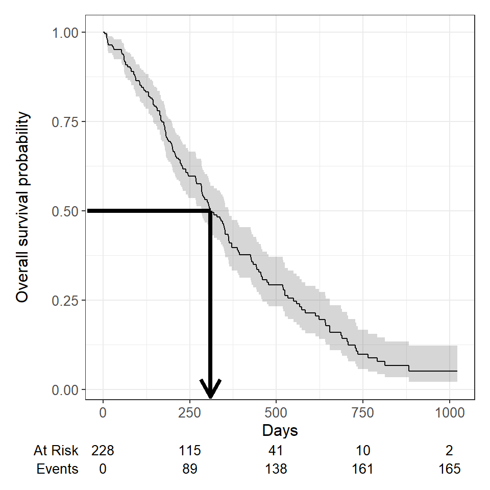
We can also get the exact median survival from our km_fit_overall object:

# Print the survfit object to see the median
print(km_fit_overall)

The output will show a median survival of 22 days, with a 95% confidence interval. This tells us that half of the patients in this dataset died within 22 days of admission.

Comparing Groups with Log-Rank Test

Next, we investigate if survival differs between patient groups. A key variable in this dataset is stroke_type (Ischaemic vs. Hemorrhagic). Let's see if there's a statistically significant difference in survival between these two groups.

Let's perform this comparison.

# Fit the Kaplan-Meier model stratified by stroke_type
km_fit_stroke_type <- survfit(Surv(time2, event_status) ~ stroke_type, data = stroke_clean)




# Plot the stratified curves
ggsurvplot(
  km_fit_stroke_type,
  data = stroke_clean,
  risk.table = TRUE,
  conf.int = TRUE,
  pval = TRUE, # Display the log-rank p-value
  legend.labs = c("Hemorrhagic", "Ischemic"),
  xlab = "Time in Days",
  ylab = "Survival Probability"
)




# You can also run the log-rank test separately
survdiff(Surv(time2, event_status) ~ stroke_type, data = stroke_clean)

The plot shows two distinct curves, with the curve for Ischemic (IS) stroke consistently above the one for Hemorrhagic (HS) stroke, suggesting better survival. The log-rank test yields a p-value of 0.03, which is statistically significant at the standard alpha=0.05 level. We can conclude that there is a significant difference in survival distributions between the two stroke types.

Step 3: Cox Proportional Hazards Regression

The log-rank test is useful, but it can't account for multiple variables simultaneously. For that, we need a regression model. The Cox Proportional Hazards model allows us to estimate the effect of several covariates while adjusting for each other.

Univariable Analysis

First, let's screen our potential predictors by fitting a univariable Cox model for each one. This helps us see the crude (unadjusted) effect of each variable. The tbl_uvregression function from {gtsummary} is perfect for this.

# Select variables for univariable analysis
univariable_models <- stroke_clean %>%
  select(sex, dm, gcs, sbp, stroke_type, referral_from, event_status, time2) %>%
  tbl_uvregression(
    method = coxph,
    y = Surv(time2, event_status),
    exponentiate = TRUE # To get Hazard Ratios
  )




# Display the table
univariable_models

The output table shows the crude Hazard Ratio for each predictor. We can see that Glasgow Coma Scale (gcs) is highly significant (p < 0.001), with an HR of 0.84. This means for each one-point increase in GCS (indicating better neurological function), the hazard of death decreases by 16%. stroke_type is also significant, as we saw with the log-rank test.

Multivariable Analysis

Now, let's build a multivariable model to see the adjusted effects. We'll include variables that were significant in the univariable analysis or are known to be clinically important. We'll use the same model as the tutorial: stroke_type, gcs, and referral_from.

# Fit the multivariable Cox model
cox_model_mv <- coxph(
  Surv(time2, event_status) ~ stroke_type + gcs + referral_from,
  data = stroke_clean
)




# Create a formatted table of the results
tbl_regression(cox_model_mv, exponentiate = TRUE)

Interpretation of the Multivariable Model:

• gcs (Glasgow Coma Scale): The adjusted HR is 0.85 (95% CI: 0.79-0.91), and it remains highly significant (p < 0.001). After accounting for stroke type and referral source, a one-point increase in GCS is associated with a 15% reduction in the hazard of death. This is our strongest predictor.
• stroke_type: The HR for IS vs. HS is 0.83 (95% CI: 0.42-1.64). The p-value is now 0.6. This means that after adjusting for the severity of the stroke (as measured by GCS) and where the patient came from, the type of stroke is no longer a statistically significant predictor of survival. This is a classic example of confounding, where the initial difference we saw was likely explained by the fact that hemorrhagic strokes tend to present with lower GCS scores.
• referral_from: The p-value is 0.5, indicating no significant difference in hazard between patients referred from a hospital versus non-hospital sources, after adjusting for the other factors.

Step 4: Checking the Proportional Hazards Assumption

The validity of our Cox model results depends on a key assumption: that the hazard ratios are constant over time. This is the Proportional Hazards (PH) assumption. We must test it.

Let's test the PH assumption for our multivariable model.

# Perform the Schoenfeld residuals test
ph_test <- cox.zph(cox_model_mv)




# Print the results
print(ph_test)

The test provides a p-value for each variable in the model and a GLOBAL p-value for the model as a whole. A p-value > 0.05 suggests that the assumption is not violated. In our case, all p-values are well above 0.05, so the statistical test indicates our model meets the PH assumption.

We can also check this visually. The plots of scaled Schoenfeld residuals should show a random scatter around a horizontal line at zero.

# Plot the residuals
ggcoxzph(ph_test)

The plots for our model variables should look relatively flat, confirming the results of the statistical test. We can be confident in our model's interpretations.

Step 5: Final Presentation and Conclusion

We have now completed a full analysis. The final step is to present our findings clearly.

Here is our final, polished model table.

tbl_regression(
  cox_model_mv,
  exponentiate = TRUE,
  pvalue_fun = ~style_pvalue(.x, digits = 3)
) %>%
  bold_p(t = 0.05) %>%
  bold_labels()

Final Synthesis:
Our analysis of the stroke dataset revealed that patient survival is strongly dependent on neurological status at admission, as measured by the Glasgow Coma Scale (GCS). For each one-point increase in GCS, the adjusted hazard of death decreased by 15%. While a non-parametric analysis suggested a survival difference between ischemic and hemorrhagic stroke types, this effect disappeared after adjusting for GCS, indicating that stroke severity, not type, was the driving factor. The final model satisfied the proportional hazards assumption, strengthening our confidence in these conclusions.

Course Conclusion

Congratulations on completing the course! You have journeyed from the foundational principles of epidemiology all the way to conducting a complete, hands-on survival analysis project.

Here are the key takeaways from today's capstone lesson, which encapsulate the entire analysis workflow:

• Always start with data preparation: Ensure your time and status variables are correctly formatted.
• Use non-parametric methods for initial exploration: Kaplan-Meier curves and log-rank tests provide a powerful, assumption-free look at survival patterns.
• Use Cox regression for multivariable analysis: This allows you to estimate adjusted effects and control for confounding.
• Always validate your model: Checking the proportional hazards assumption is a non-negotiable step for a valid Cox model.
• Interpretation is key: The ultimate goal is to translate statistical output into meaningful insights.

You now have a solid foundation and a practical skillset in both epidemiological study design and survival analysis. From here, your data science journey could take you into more advanced topics like machine learning models for survival prediction, analyzing recurrent or competing events in greater detail, or designing complex clinical trials. Well done, and best of luck in your future analyses