Cox Proportional Hazards Modeling in R

Welcome back! In our last session, we mastered the log-rank test, a powerful tool for determining if a statistically significant difference exists between survival curves. However, we also highlighted its key limitations: it doesn't quantify the size of the difference, nor can it account for the influence of multiple variables at once.

This lesson introduces the solution: the Cox Proportional Hazards model. This is one of the most widely used regression models in survival analysis. You will learn how to fit a Cox model in R using the survival package and, most importantly, how to interpret its output to understand the effect of different factors on survival. This moves us from simply asking "is there a difference?" to "how large is the difference, and what factors are driving it?".

From Univariate Comparison to Multivariate Modeling

The log-rank test is a univariate method; it compares survival based on a single categorical factor (e.g., treatment group, gender). In real-world data, survival is often influenced by many factors simultaneously. For instance, a difference in survival between two treatment groups might actually be due to one group being older on average. The Cox model allows us to perform a multivariate analysis, assessing the impact of one variable while statistically adjusting for the effects of others.

The following resource provides a great introduction to why we need a model like the Cox model to move beyond the limitations of the log-rank test.

Cox Proportional-Hazards Model - Easy Guides - Wiki - STHDA

This article from STHDA clearly explains the motivation for using the Cox model.

Start by reading the introduction, from the initial description. Then, move to the section "Why is it important?" and read the first two paragraphs, which explain the need to adjust for multiple factors.

The core output of a Cox model is the Hazard Ratio (HR), which quantifies the effect of a covariate on the rate of events (the hazard). This is the effect size measure that the log-rank test lacks.

The Cox Model Formula and the Hazard Ratio

The mathematical form of the Cox model helps clarify what it does. The model expresses the hazard at time $t$ for an individual with a specific set of covariates.

h (t) = h_{0} (t) \times exp (b_{1} x_{1} + b_{2} x_{2} + \dots + b_{p} x_{p})

Let's break this down intuitively:

$h (t)$ is the hazard (instantaneous risk of event) for an individual at time $t$ .
$h_{0} (t)$ is the baseline hazard. This is the hazard when all covariate values ( $x_{1}, x_{2}, \dots$ ) are zero. The model is called "semi-parametric" because it makes no assumption about the shape of this baseline hazard function.
$exp (b_{1} x_{1} + \dots)$ is the part that adjusts the baseline hazard based on an individual's covariate values.

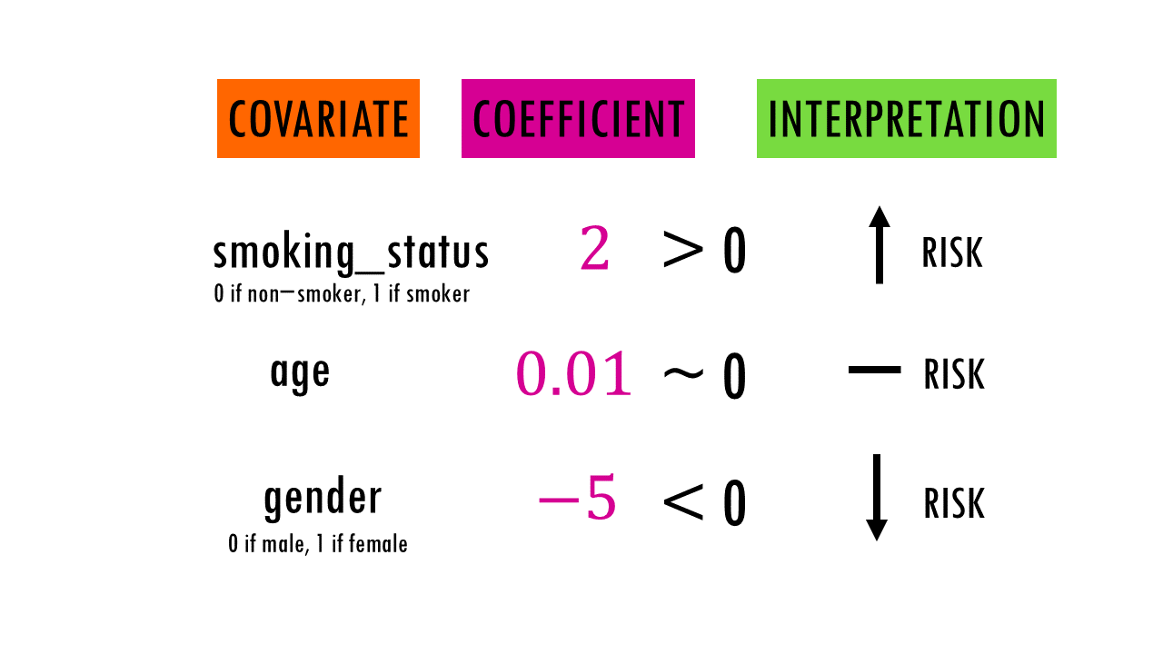
The key quantities we interpret are the Hazard Ratios (HR), which are the exponentiated coefficients ( $exp (b_{i})$ ).

HR = 1: The covariate has no effect on the hazard.
HR > 1: The covariate is associated with an increased hazard (worse survival).
HR < 1: The covariate is associated with a decreased hazard (better survival).

This image illustrates how the sign and magnitude of a coefficient relate to its effect on risk. A positive coefficient (HR > 1) increases risk, a negative coefficient (HR < 1) decreases risk, and a coefficient near zero (HR ~ 1) has no significant effect.

Fitting and Interpreting a Cox Model in R

Fitting a Cox model in R uses the coxph() function from the survival package. The syntax is very similar to other modeling functions in R and to the survfit() function you've already used.

Let's start by fitting a univariable model for the effect of sex in the lung dataset. This is analogous to the log-rank test we ran in the previous lesson.




# Load the necessary libraries
library(survival)
library(survminer)




# Fit a univariable Cox model for the 'sex' variable
# Note: In the lung dataset, sex=1 is male, sex=2 is female.
# R automatically uses the first level (male) as the reference.
cox_uni <- coxph(Surv(time, status) ~ sex, data = lung)




# Display a summary of the model results
summary(cox_uni)

This produces the following output:

Call:
coxph(formula = Surv(time, status) ~ sex, data = lung)

  n= 228, number of events= 165 

         coef exp(coef) se(coef)      z Pr(>|z|)   
sex   -0.5310    0.5880   0.1672 -3.176  0.00149 **
---
Signif. codes:  0 ‘***’ 0.001 ‘**’ 0.01 ‘*’ 0.05 ‘.’ 0.1 ‘ ’ 1

      exp(coef) exp(-coef) lower .95 upper .95
sex     0.588      1.701    0.4237    0.8163

Concordance= 0.579  (se = 0.022 )
Likelihood ratio test= 10.63  on 1 df,   p=0.001
Wald test            = 10.09  on 1 df,   p=0.001
Score (logrank) test = 10.33  on 1 df,   p=0.001

This output is information-rich. The following video provides a fantastic walkthrough of how to interpret each part.

Survival Analysis Part 11 | Cox Proportional Hazards Model in R with RStudio

The "MarinStatsLectures" channel provides an exceptionally clear explanation of the summary(coxph) output. Watching this will solidify your understanding of each component.

Please watch the section that explains how to interpret the summary of the model. The lecturer breaks down the coefficients, hazard ratios, confidence intervals, and the meaning of exp(-coef).

Let's recap the key points from the video and the R output:

coef (-0.5310): This is the estimated regression coefficient ( $b$ ) for the sex variable. It's on a log-hazard scale, so it's not directly interpretable. Its negative sign indicates a protective effect for the non-reference group (females).
exp(coef) (0.5880): This is the Hazard Ratio (HR). This is the most important number for interpretation.
- Interpretation: Females (sex=2) have a hazard of death that is 0.588 times that of males (sex=1) at any given point in time.
- Percentage Change: You can also say that females have a (1 - 0.588) = 41.2% lower hazard of death compared to males.
Pr(>|z|) (0.00149): This is the p-value for the coefficient. Since it is less than 0.05, we conclude that the effect of sex is statistically significant.
lower .95, upper .95 (0.4237, 0.8163): This is the 95% confidence interval for the Hazard Ratio. Since this interval does not contain 1, it confirms that the result is statistically significant. We are 95% confident that the true hazard ratio for females vs. males lies between 0.42 and 0.82.
Score (logrank) test (p=0.001): Notice that the p-value for the Score test is the same as the one we got from the survdiff() log-rank test in the previous lesson. A univariable Cox model is mathematically related to the log-rank test.

Multivariable Cox Regression: Adjusting for Confounders

The real power of the Cox model comes from including multiple variables. Let's build a model that includes sex, age, and physician-rated performance status (ph.ecog).




# Fit a multivariable Cox model
# We must remove missing values first for the model to run
lung_complete <- na.omit(lung) 

cox_multi <- coxph(Surv(time, status) ~ age + sex + ph.ecog, data = lung_complete)

summary(cox_multi)

Call:
coxph(formula = Surv(time, status) ~ age + sex + ph.ecog, data = lung_complete)

  n= 167, number of events= 119
   (61 observations deleted due to missingness)

             coef exp(coef) se(coef)      z Pr(>|z|)    
age       0.01724   1.01739  0.01010  1.706   0.0879 .  
sex      -0.57949   0.56019  0.20572 -2.817   0.0048 ** 
ph.ecog   0.62734   1.87262  0.13689  4.583 4.59e-06 ***
---
Signif. codes:  0 ‘***’ 0.001 ‘**’ 0.01 ‘*’ 0.05 ‘.’ 0.1 ‘ ’ 1

        exp(coef) exp(-coef) lower .95 upper .95
age        1.0174     0.9829    0.9976    1.0376
sex        0.5602     1.7851    0.3753    0.8361
ph.ecog    1.8726     0.5340    1.4312    2.4491

...

Let's interpret this adjusted model.

sex (HR = 0.56, p = 0.0048): After adjusting for age and ECOG score, females still have a significantly lower hazard of death compared to males. The hazard is about 44% lower (1 - 0.56). Notice the HR and p-value are slightly different from the univariable model; this is the effect of adjustment.
age (HR = 1.017, p = 0.088): This is a continuous variable.
- Interpretation: For each one-year increase in age, the hazard of death increases by a factor of 1.017 (or about 1.7%), holding sex and ECOG score constant.
- This effect is not statistically significant at the 0.05 level (p=0.088).
ph.ecog (HR = 1.87, p < 0.001): This is a numeric score where higher values mean worse performance status.
- Interpretation: For each one-unit increase in the ECOG score, the hazard of death increases by a factor of 1.87 (or 87%), holding age and sex constant. This is a very strong and significant predictor of survival.

The following practical guide demonstrates fitting and interpreting both univariable and multivariable models, reinforcing these concepts.

Cox Proportional-Hazards Model - Easy Guides - Wiki - STHDA

This guide walks through the entire process of fitting and interpreting both simple and complex Cox models in R.

First, read the subsection Univariate Cox regression to see a detailed interpretation of a single-predictor model. Then, read the next subsection on Multivariable Cox regression to understand how the interpretation changes when you adjust for multiple factors.

The Proportional Hazards Assumption

The Cox model is powerful, but it relies on a critical assumption: the proportional hazards assumption. This means that the effect of a covariate (i.e., the hazard ratio) is constant over time. For example, if the HR for females vs. males is 0.5, this assumption implies that the hazard for females is half that of males throughout the entire follow-up period. If the effect of a variable changes over time (e.g., a drug is very effective early on but its benefit diminishes later), the assumption is violated.

Visually, this means the survival curves for different groups should have a roughly parallel trend and should not cross. Checking this assumption is a critical step in any Cox model analysis.

Conclusion

In this lesson, you have taken a major step forward in survival analysis, moving from simple comparisons to sophisticated regression modeling. You are now equipped to fit and interpret the workhorse of survival analysis, the Cox proportional hazards model.

Key takeaways from today's lesson:

The Cox model allows for multivariate survival analysis, quantifying the effect of predictors as Hazard Ratios (HR) while adjusting for confounders.
In R, the coxph() function from the survival package is used to fit the model.
An HR > 1 indicates increased risk, while an HR < 1 indicates decreased risk. The p-value and confidence interval tell you if this effect is statistically significant.
The interpretation of an HR for a given variable is always conditional on the other variables in the model ("holding other factors constant").
The model depends on the crucial proportional hazards assumption, which states that the effect of a covariate is constant over time.

In our next lesson, we will focus entirely on this crucial assumption. You will learn how to use graphical methods and formal statistical tests in R to diagnose whether the proportional hazards assumption holds for your model, and what to do if it doesn't.