Log-Rank Test in R

What Question Does the Log-Rank Test Answer?

When we look at two Kaplan-Meier curves, like the ones for males and females from our last session, they might appear different. But is that difference "real" in a statistical sense, or could it have just occurred by chance? The log-rank test provides a formal way to answer this.

Its core purpose is to test a specific hypothesis about the survival distributions of the groups being compared. The following article provides a very clear, non-mathematical explanation of this.

The key hypotheses are:

• Null Hypothesis ($H_0$): There is no difference in survival between the groups. The survival curves are identical in the populations from which the samples were drawn.
• Alternative Hypothesis ($H_A$): There is a difference in survival between the groups. The survival curves are not identical.

This can be visualized quite simply. Under the null hypothesis, the curves for different groups would essentially overlap. Under the alternative hypothesis, they would be distinct.

The Intuition: Observed vs. Expected Events

So, how does the test decide between these two hypotheses? You don't need to perform the calculations by hand, but understanding the logic is crucial for interpretation, especially given your interest in the "why" behind the methods.

At its heart, the log-rank test is a type of chi-square test. For each time an event (e.g., a death) occurs, the test calculates:

1. The observed number of events in each group.
2. The expected number of events in each group, assuming the null hypothesis is true (i.e., assuming the risk is the same for everyone, regardless of group).

It then sums these observed and expected counts across all event times and compares them. If the total observed events in each group are very different from what was expected, this suggests the null hypothesis is wrong. The chi-square statistic quantifies this difference, which is then converted into a p-value.

Let's read a brief, intuitive summary of this process.

If you are curious to see a step-by-step numerical example of this observed vs. expected calculation, the following optional video provides a great walkthrough.

Performing the Log-Rank Test in R

In R, the primary function for this test is survdiff() from the survival package. Its structure is very similar to the survfit() function you're already familiar with.

Let's revisit the lung dataset and formally test the difference in survival between males and females that we plotted in our last lesson.

Now, let's apply this to our lung data.

# Load libraries if not already loaded
library(survival)
library(survminer)




# Perform the log-rank test comparing survival by sex
# The formula `Surv(time, status) ~ sex` is the same one we used for plotting
logrank_test_sex <- survdiff(Surv(time, status) ~ sex, data = lung)




# Print the results
print(logrank_test_sex)

This produces the following output:

Call:
survdiff(formula = Surv(time, status) ~ sex, data = lung)

        N Observed Expected (O-E)^2/E (O-E)^2/V
sex=1 138      112     91.4      4.65      10.3
sex=2  90       53     73.6      5.77      10.3

 Chisq= 10.3  on 1 degrees of freedom, p= 0.001 

Interpreting the Output

Let's break down this output piece by piece:

• N: The number of subjects in each group (138 males, 90 females).
• Observed: The actual number of events (deaths) observed in each group. We saw 112 deaths among males and 53 among females.
• Expected: The number of deaths we would have expected in each group if the null hypothesis were true. We expected 91.4 deaths for males but saw 112. We expected 73.6 for females but saw only 53. This discrepancy is the evidence against the null hypothesis.
• (O-E)^2/E: A component of the chi-square calculation for each group.
• Chisq= 10.3: The overall chi-square test statistic, which summarizes the total difference between observed and expected counts across both groups.
• on 1 degrees of freedom: The degrees of freedom is the number of groups minus 1 (i.e., 2 - 1 = 1).
• p= 0.001: This is the final result. It is the probability of observing a difference this large (or larger) between the survival curves if there were truly no difference in the populations.

Since our p-value (0.001) is much smaller than the conventional significance level of 0.05, we reject the null hypothesis. We can conclude that there is a statistically significant difference in survival time between males and females in this dataset.

The following resource provides a concise guide to interpreting p-values from this test.

As you saw in the previous lesson, the ggsurvplot function can run this test for you and add the p-value directly to the plot by setting pval = TRUE. This is often the most efficient workflow, as it combines the formal test with the visualization.

Comparing More Than Two Groups

The log-rank test is not limited to two groups. We can use it to compare three or more groups simultaneously. For example, let's compare survival across different physician-rated ECOG performance scores (ph.ecog) in the lung dataset.

The hypotheses are slightly different in this case:

• Null Hypothesis ($H_0$): The survival curves for all groups are identical.
• Alternative Hypothesis ($H_A$): At least one of the survival curves is different from the others.

A significant p-value tells you that the groups are not all the same, but it does not tell you which specific groups differ from each other (similar to an ANOVA F-test in regression).

# Perform a log-rank test for the ph.ecog variable (ECOG performance score)
# Note: some values are missing, so we'll filter them out first.
lung_filtered <- lung[!is.na(lung$ph.ecog), ]

logrank_test_ecog <- survdiff(Surv(time, status) ~ ph.ecog, data = lung_filtered)

print(logrank_test_ecog)

Call:
survdiff(formula = Surv(time, status) ~ ph.ecog, data = lung_filtered)

             N Observed Expected (O-E)^2/E (O-E)^2/V
ph.ecog=0   63       37     52.3      4.52      6.47
ph.ecog=1  113       82     87.3      0.32      0.65
ph.ecog=2   51       44     27.1     10.56     14.88
ph.ecog=3    1        1      0.3      1.59      1.61

 Chisq= 21.8  on 3 degrees of freedom, p= 7e-05 

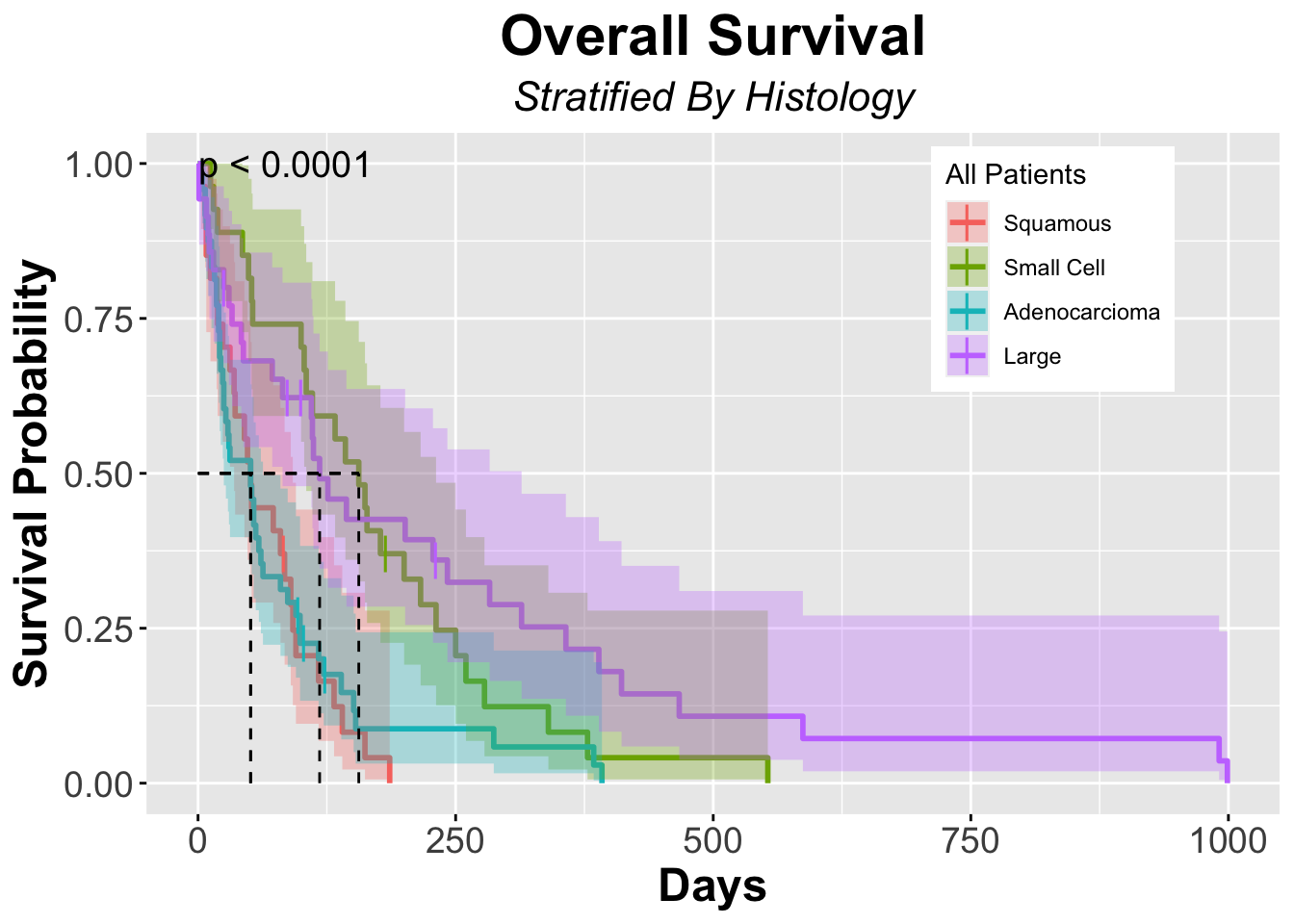
The very small p-value (p= 7e-05, or 0.00007) indicates a highly significant difference in survival among the different ECOG performance score groups. Looking at the plot gives us the visual context for this result.

Limitations and Looking Ahead

The log-rank test is a fundamental tool, but it has two key limitations:

1. It tells you if a difference exists, but it doesn't quantify the size of that difference (e.g., how much better is survival in one group compared to another?).
2. It's a simple comparison of groups and cannot adjust for other variables (confounders). For example, if one treatment group is older on average than another, the log-rank test can't separate the effect of the treatment from the effect of age.

These limitations bring us directly to the need for a more powerful tool: regression modeling for survival data.

Conclusion

In this lesson, you've moved beyond visual inspection to statistically test the differences between survival curves. You now understand the conceptual basis of the log-rank test and can confidently perform and interpret it in R.

Here are the main takeaways:

• The log-rank test is a hypothesis test that formally compares survival distributions among two or more independent groups.
• The null hypothesis states that there is no difference in survival between the groups.
• The test works by comparing the observed number of events to the expected number of events under the null hypothesis.
• In R, the survdiff() function performs the test, and its primary output for interpretation is the p-value.
• A significant p-value indicates that at least one group's survival distribution is different from the others, but it does not quantify the size of the effect or adjust for confounders.

The limitations of the log-rank test perfectly set the stage for our next lesson, where we will explore the Cox Proportional Hazards Model. This regression model will allow us to not only compare groups but also to estimate the magnitude of the effect (the Hazard Ratio) and adjust for multiple covariates simultaneously.