Kaplan-Meier Curves in R

A Refresher on Interpreting Kaplan-Meier Curves

Before we start coding, let's quickly refresh our understanding of what a Kaplan-Meier (KM) curve shows and how to interpret it. These curves are the standard method for visualizing survival data, especially when it includes censored observations.

This short video provides an excellent overview of how to read a KM curve, which is exactly what we are about to create in R.

Setting Up for Survival Analysis in R

To perform survival analysis in R, we'll rely on two key packages. Your CIS background gives you a good handle on the modular nature of software, and in R, this is managed through packages that provide specialized functions.

1. survival: This is the foundational package for survival analysis in R. It contains the core functions for creating survival objects and fitting models like Kaplan-Meier and Cox regression. It comes with the base R installation, so you don't need to install it, but you do need to load it.
2. survminer: This package excels at creating highly customizable and publication-ready visualizations of survival analysis results, building on the popular ggplot2 graphics system.

You will need to install survminer if you haven't already, and then load both packages into your R session.

# Install the survminer package if you don't have it
install.packages("survminer")

# Load the necessary packages for this session
library(survival)
library(survminer)

For our examples, we will use the lung dataset, which is included in the survival package. It contains data on survival in patients with advanced lung cancer.

The two most important columns for us will be:

• time: The survival time in days.
• status: The censoring status. Note the coding here: 1 means the observation was censored, and 2 means the event (death) occurred. This is a common convention but can be counter-intuitive, so it's important to always check the data documentation.

The Core Components: Surv() and survfit()

The survival package uses a specific workflow that centers on two functions:

1. Surv(): This function creates a special "survival object." From your data structures experience, you can think of this as a composite object that bundles the time-to-event and the event/censoring indicator together. This is the standard format for the response variable in all survival models in R.

2. survfit(): This is the function that does the actual work of calculating the Kaplan-Meier estimate. It takes a formula as input, with the Surv() object as the response.

Let's see this in action. The following guide provides clear code examples for these steps.

First, let's create a survfit object for the overall survival in the lung dataset. The formula Surv(time, status) ~ 1 tells R to calculate a single survival curve for the whole cohort, without any grouping variables.

# Fit a Kaplan-Meier model for the entire cohort
sfit_overall <- survfit(Surv(time, status) ~ 1, data = lung)

# Print the object to see a summary
print(sfit_overall)

The output gives you a quick summary:

Call: survfit(formula = Surv(time, status) ~ 1, data = lung)

      n  events  median 0.95LCL 0.95UCL
    228     165     310     285     363 

Interpretation:

• n: 228 patients in the study.
• events: 165 deaths were observed.
• median: The median survival time is 310 days. This means half of the patients survived longer than 310 days, and half survived less.
• 0.95LCL, 0.95UCL: The 95% confidence interval for the median survival is between 285 and 363 days.

More interestingly, we can compare survival between groups. Let's create survfit object stratified by sex.

# Fit Kaplan-Meier curves stratified by sex
sfit_by_sex <- survfit(Surv(time, status) ~ sex, data = lung)

# Print the summary
print(sfit_by_sex)

Call: survfit(formula = Surv(time, status) ~ sex, data = lung)

        n events median 0.95LCL 0.95UCL
sex=1 138    112    270     212     310
sex=2  90     53    426     348     550

This output now shows the same summary but broken down for males (sex=1) and females (sex=2). We can immediately see a difference in median survival: 270 days for males vs. 426 days for females. Now, let's visualize this difference.

Plotting and Interpreting with ggsurvplot

While you can use base R's plot() function, the ggsurvplot() function from the survminer package provides a far richer and more intuitive visualization. It can automatically add confidence intervals, risk tables, and other crucial elements for interpretation.

The following resource walks through creating a detailed plot.

Let's build a comprehensive plot for our sfit_by_sex object.

# Create a detailed survival plot using ggsurvplot
ggsurvplot(
  sfit_by_sex, 
  data = lung,
  pval = TRUE,            # Add log-rank p-value
  conf.int = TRUE,        # Add confidence intervals
  risk.table = TRUE,      # Add a table of numbers at risk
  surv.median.line = "hv",# Add median survival lines
  legend.labs = c("Male", "Female"), # Change legend labels
  ggtheme = theme_bw()    # Use a clean black-and-white theme
)

This single command generates a rich, multi-panel plot that contains nearly all the information you need for a thorough interpretation.

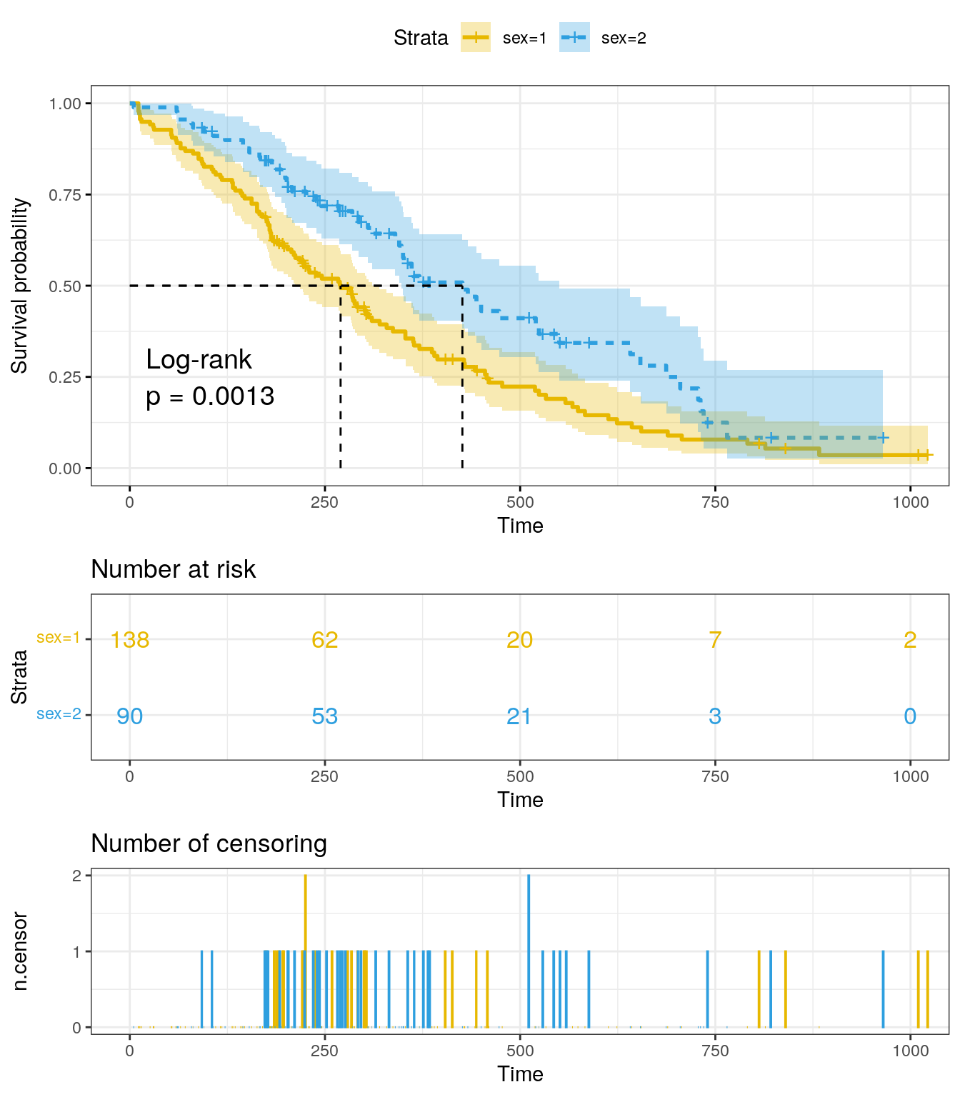
This is an example of a comprehensive Kaplan-Meier plot, similar to the one our code generates. It includes survival curves for two groups with confidence intervals, a log-rank p-value, a "Number at risk" table, and a plot showing the "Number of censoring" events over time.

Let's break down how to interpret this plot, referring to the image above as our guide:

• Axes: The y-axis is the probability of survival, starting at 1.0 (100%). The x-axis is time.
• Curves: Each colored line represents a group (e.g., males and females). A curve that is consistently higher indicates better survival. Here, the blue curve (sex=2, Female) is above the yellow curve (sex=1, Male), suggesting females have a better survival probability over time.
• Vertical Drops: Each time a curve drops, it signifies that one or more events (deaths) occurred at that time point.
• Crosses/Tick Marks: The small + symbols on the curves represent censored observations. At these time points, a patient was lost to follow-up or the study ended, but they had not experienced the event. They contribute information up to that point.
• Confidence Bands: The shaded areas around each curve represent the 95% confidence interval. Wider bands indicate more uncertainty in the survival estimate, which usually happens later in the study when fewer patients are left.
• Median Survival: The dashed lines show the median survival for each group—the time at which survival probability drops to 0.5 (50%). You can see the median survival for the yellow group is ~270 days, while for the blue group, it's ~426 days.
• P-value: The "Log-rank p = 0.0013" tells us that the observed difference between these two curves is statistically significant. We will explore the log-rank test in detail in our next lesson.

• Number at Risk Table: This is a critical component. It shows how many patients were still alive and being followed (at risk) in each group at specific time points. It provides context for the stability of the curves. For example, you can see the number of patients diminishes over time due to both events and censoring.

Conclusion

In this lesson, you've successfully transitioned from theoretical knowledge to practical application in survival analysis. You have learned the complete workflow for generating and interpreting Kaplan-Meier survival curves in R, a cornerstone skill for analyzing time-to-event data.

Key takeaways from today's session include:

• The survival and survminer packages are the primary tools for survival analysis and visualization in R.
• The workflow involves creating a Surv object to encapsulate time and event data, fitting a model with survfit(), and visualizing the result with ggsurvplot().
• A comprehensive Kaplan-Meier plot includes not just the curves, but also confidence intervals, a p-value, and a risk table, all of which are essential for a full interpretation.
• You can now read a KM plot to compare survival between groups, estimate median survival, and understand the impact of censoring.

In our plot, we included a p-value from a log-rank test. In the next lesson, we will delve into the theory and practice of the log-rank test, learning how to formally compare survival distributions between two or more groups and interpret the results.