Gradients: Vectors of Partial Derivatives

Hello! Welcome back to our course on the mathematical foundations for machine learning.

In our last lesson, we explored how the derivative of a single-variable function, $f (x)$ , gives us its instantaneous rate of change. We saw that by finding where the derivative equals zero, we can locate the minimum or maximum points of a function. This is the key to optimization, like finding the single parameter $w$ that minimizes a loss function $L (w)$ .

However, real machine learning models are rarely this simple. Their loss functions depend on not just one, but thousands or even millions of parameters (weights and biases). This means we're dealing with multi-variable functions, like $L (w_{1}, w_{2}, w_{3}, ...)$ . So, how do we find the "slope" on a high-dimensional surface to know which way is "downhill"?

Today, we'll answer that question. Our goal is to describe the concept of a gradient as a vector of partial derivatives for multi-variable functions. The gradient is the multi-dimensional equivalent of the derivative, and it is the single most important tool for training modern machine learning models.

From a Curve to a Surface

With a single-variable function like $y = f (x)$ , we can visualize it as a curve on a 2D plane. A multi-variable function, such as $z = f (x, y)$ , is best visualized as a 3D surface, like a landscape with hills and valleys. The height of the landscape at any coordinate (x, y) is given by the value of the function z.

When standing on such a surface, the slope is no longer a single number. The steepness depends entirely on the direction you choose to move. Moving along the x-axis might be a gentle slope, while moving along the y-axis might be very steep.

To build an intuition for this, let's watch a short video that visualizes a multi-variable function as a temperature "hill" on a metal plate.

Best Explanation of Partial Derivatives and Gradients

The video 'Best Explanation of Partial Derivatives and Gradients' from Brain Station Advanced provides an excellent visualization of a multi-variable function.

Watch the beginning of the video from 00:00 to 01:54. Focus on how the temperature on a 2D plate can be represented as a 3D hill, where the height represents the temperature. This is the mental model we'll use for a multi-variable function.

Partial Derivatives: Slopes in Specific Directions

To handle the complexity of slopes in multiple directions, we can simplify the problem. Instead of trying to find the slope in every direction at once, we can ask: what is the slope if we only move along one specific axis, while holding all other variables constant?

This is the core idea of a partial derivative.

Imagine you are on that 3D landscape. To find the partial derivative with respect to $x$ , you would face the x-direction and measure the slope of the ground in front of you, ignoring any changes to your left or right (in the y-direction). Geometrically, this is like taking a vertical "slice" of the 3D surface parallel to the x-axis and finding the slope of the resulting 2D curve.

We use the symbol $\partial$ (a "curly d") to denote a partial derivative. The partial derivative of $f$ with respect to $x$ is written as $\frac{\partial f}{\partial x}$ .

The great thing is that calculating a partial derivative uses the same differentiation rules you already know. The key trick is to treat all other variables as constants.

This video provides a clear explanation and a worked-out example of how to compute partial derivatives.

Partial Derivatives and the Gradient of a Function

Let's watch a segment from 'Partial Derivatives and the Gradient of a Function' by Professor Dave Explains. It clearly demonstrates the process of calculating partial derivatives.

Watch from 02:30 to 05:17. Pay close attention to how, when differentiating with respect to 'x', the variable 'y' is treated just like a constant number. Then, see how the roles are reversed when differentiating with respect to 'y'.

The Gradient: The Direction of Steepest Ascent

We've now seen how to find the rate of change along each individual axis using partial derivatives.

$\frac{\partial f}{\partial x}$ gives the rate of change in the x-direction.
$\frac{\partial f}{\partial y}$ gives the rate of change in the y-direction.

But what if we want to find the direction of the steepest possible uphill slope at a given point? This is what the gradient gives us.

The gradient is simply a vector that collects all the partial derivatives of a function. For a two-variable function $f (x, y)$ , the gradient, denoted by $\nabla f$ (pronounced "nabla f" or "del f"), is:

\nabla f (x, y) = [\frac{\partial f}{\partial x} \frac{\partial f}{\partial y}]

This vector has two crucial properties:

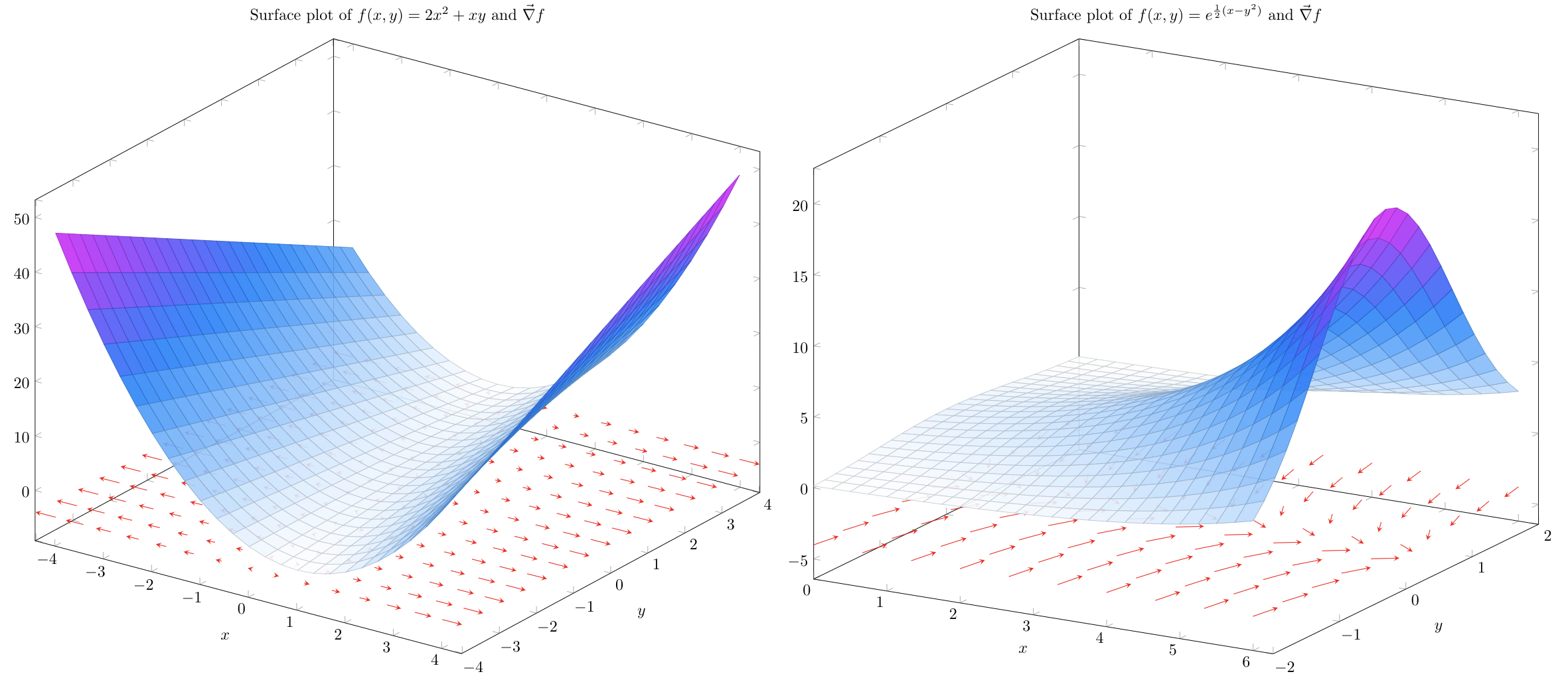
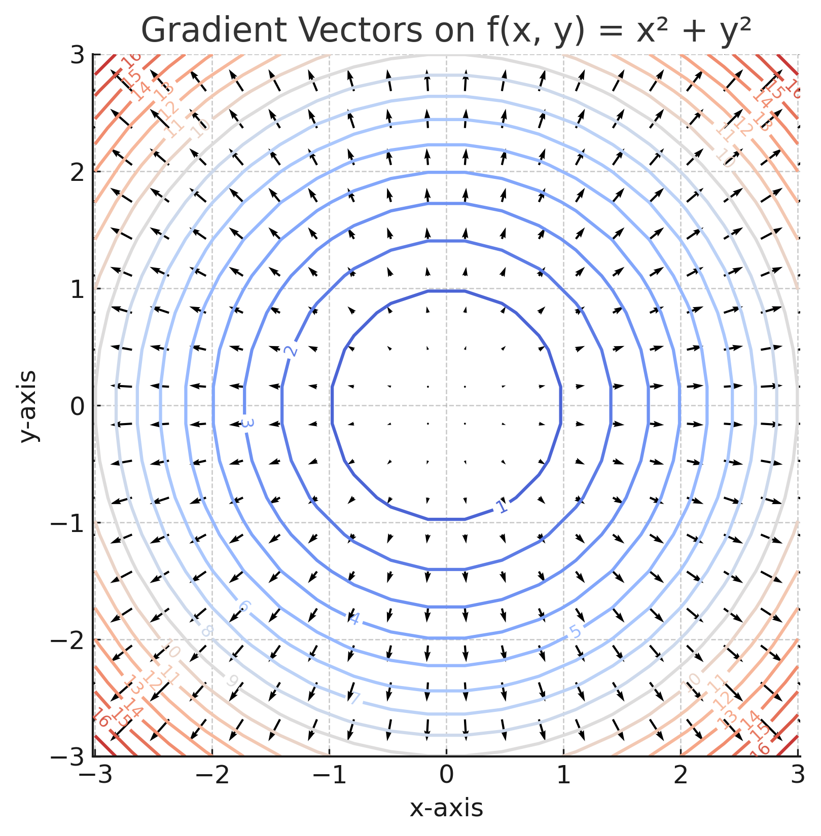
Direction: It points in the direction of the steepest ascent of the function at that point.
Magnitude: Its length (magnitude) represents the rate of change in that steepest direction. A large magnitude means the hill is very steep; a small magnitude means it's nearly flat.

The following images provide a powerful visual for this concept.

Surface Plots with Gradient Vector Fields — This image shows two functions as 3D surfaces. The red arrows on the 2D plane below each surface represent the gradient vectors. Notice how they always point "uphill," away from the valleys and towards the peaks.

Gradient Vectors on f(x, y) = x² + y² — Here, the function is shown as a 2D contour plot, where lines connect points of equal height. The gradient vectors (arrows) are always perpendicular to the contour lines and point towards higher-valued contours—the direction of steepest ascent.

Let's solidify this idea by reading a concise summary.

Partial Derivatives & Gradients | AI Under the Hood (Beta)

The article 'Partial Derivatives & Gradients' on AI Under the Hood neatly summarizes the definition and meaning of the gradient vector.

Read section 4, 'The Gradient Vector.' It formally defines the gradient and introduces the excellent analogy of the gradient being a 'compass in parameter space' for finding minima.

The Gradient's Role in Machine Learning

Now we can connect everything back to our goal of training machine learning models. The loss function of a model is a high-dimensional surface, and we want to find its lowest point.

The gradient, $\nabla L$ , at any set of parameters points in the direction that increases the loss the fastest. To minimize the loss, we should therefore take a small step in the opposite direction of the gradient.

This simple but powerful idea is the basis for gradient descent, the most common optimization algorithm in machine learning. We will dedicate a future module to it, but now you understand its fundamental component. By repeatedly calculating the gradient and taking steps "downhill," we can iteratively update our model's parameters to minimize the loss and find the best-performing model.

Test your understanding!

Consider the function $f (x, y) = 2 x^{3} + 5 y^{2}$ .

Find the partial derivative with respect to $x$ , $\frac{\partial f}{\partial x}$ .
Find the partial derivative with respect to $y$ , $\frac{\partial f}{\partial y}$ .
Write down the gradient vector, $\nabla f$ .
Calculate the gradient vector at the point $(x = 1, y = 2)$ . What does this vector tell you?

Show answer

Partial derivative with respect to $x$ : Treat $y$ as a constant. The derivative of $2 x^{3}$ is $6 x^{2}$ . The derivative of the constant term $5 y^{2}$ is 0.
$\frac{\partial f}{\partial x} = 6 x^{2}$
Partial derivative with respect to $y$ : Treat $x$ as a constant. The derivative of the constant term $2 x^{3}$ is 0. The derivative of $5 y^{2}$ is $10 y$ .
$\frac{\partial f}{\partial y} = 10 y$
Gradient vector: Combine the partial derivatives into a vector.
$\nabla f = [6 x^{2} 10 y]$
Gradient at $(1, 2)$ : Substitute $x = 1$ and $y = 2$ into the gradient vector formula.
$\nabla f (1, 2) = [6 (1)^{2} 10 (2)] = [620]$
Interpretation: At the point $(1, 2)$ on the surface defined by $f (x, y)$ , the direction of steepest ascent is given by the vector $[620]$ . This means to go uphill the fastest, you should move 6 units in the positive x-direction for every 20 units you move in the positive y-direction.

Conclusion

In this lesson, we successfully extended the concept of a derivative to functions with multiple variables. This is a huge step toward understanding how large-scale machine learning models are trained.

Here are our key takeaways:

For multi-variable functions, we can't talk about a single slope. The slope depends on the direction of movement.
A partial derivative measures the rate of change along one specific axis, while treating all other variables as constants.
The gradient ( $\nabla f$ ) is a vector composed of all the partial derivatives of a function.
The gradient vector always points in the direction of the steepest increase of the function, and its magnitude represents the steepness of that slope.
In machine learning, we move in the direction opposite to the gradient of the loss function to find its minimum.

We've now covered derivatives and gradients. In our next lesson, we will focus on basic vector and matrix operations. These operations are the language of linear algebra and are essential for efficiently handling data and performing the calculations, like computing gradients, on the massive scale required by modern AI.

Recommended resources

From a Curve to a Surface

Partial Derivatives: Slopes in Specific Directions

The Gradient: The Direction of Steepest Ascent

The Gradient's Role in Machine Learning

Conclusion