Vector and Matrix Operations Fundamentals

Hello! Welcome back to our course on the mathematical foundations for machine learning.

In our last lesson, we saw that the gradient of a multi-variable function is a vector pointing in the direction of the steepest ascent. This is a powerful concept, but to actually use it for training models—and to handle data in general—we need a toolkit for working with these vectors and their close relatives, matrices.

Today's lesson provides that toolkit. Our learning outcome is to apply basic vector and matrix operations, including dot products and matrix-vector multiplication. We'll cover the essential arithmetic of linear algebra that forms the computational engine of virtually all machine learning algorithms. You'll see how these operations allow us to efficiently process data and update model parameters.

Vectors and Matrices in Machine Learning

First, let's solidify what we mean by vectors and matrices in a practical ML context.

A vector is an ordered list of numbers. It can represent:
- A single data point with multiple features (e.g., [age, income, years_of_experience]).
- The parameters of a simple model.
- The gradient of a loss function, as we saw previously.
A matrix is a rectangular grid of numbers, which you can think of as a collection of vectors. It can represent:
- An entire dataset, where each row is a data point (a vector) and each column is a feature.
- The weights of a neural network layer, connecting multiple inputs to multiple outputs.

These are the fundamental objects we manipulate in machine learning. Let's learn how to manipulate them.

Basic Vector Operations

The simplest operations involve working with one or two vectors. They are performed element-wise, meaning the operation applies to corresponding elements in the vectors.

To see how this works, let's watch the beginning of the following video. It covers vector-scalar multiplication and vector addition.

ML Zoomcamp 1.8 - Linear Algebra Refresher

This clip from 'ML Zoomcamp - Linear Algebra Refresher' by DataTalksClub provides a quick, practical demonstration of element-wise vector operations.

Watch from 00:14 to 02:21. Notice how multiplying a vector by a number (a scalar) scales each element individually, and adding two vectors combines them element by element.

As the video shows:

Vector-Scalar Multiplication: Multiplying a vector by a single number (a scalar) scales its magnitude. If $v = [v_{1}, v_{2}, v_{3}]$ and $c$ is a scalar, then $c v = [c v_{1}, c v_{2}, c v_{3}]$ .
Vector Addition: Adding two vectors of the same size results in a new vector where each element is the sum of the elements at the same position. If $u = [u_{1}, u_{2}, u_{3}]$ and $v = [v_{1}, v_{2}, v_{3}]$ , then $u + v = [u_{1} + v_{1}, u_{2} + v_{2}, u_{3} + v_{3}]$ .

The Dot Product: Measuring Alignment

A more interesting operation is the dot product (also called inner product). Unlike the previous operations, it takes two vectors and returns a single number (a scalar).

Mechanics: The dot product is the sum of the products of corresponding elements.
For vectors $a = [a_{1}, a_{2}, \dots, a_{n}]$ and $b = [b_{1}, b_{2}, \dots, b_{n}]$ , their dot product is:
$a \cdot b = a_{1} b_{1} + a_{2} b_{2} + \dots + a_{n} b_{n} = \sum_{i = 1}^{n} a_{i} b_{i}$

Intuition: The dot product measures the "alignment" or "similarity" between two vectors. This idea is fundamental in machine learning.

To build this intuition, let's read a short, clear explanation.

Why Deep Learning Loves the Dot Product and Matrix ...

The article 'Why Deep Learning Loves the Dot Product' provides an excellent geometric interpretation of what the dot product represents.

Read the first section, 'The Essence of the Dot Product.' Focus on the three cases that illustrate how the dot product's value (positive, zero, or negative) relates to the angle between the vectors.

To summarize the key insight:

Large positive dot product: The vectors point in a similar direction.
Dot product near zero: The vectors are nearly perpendicular (orthogonal), indicating no alignment.
Large negative dot product: The vectors point in opposite directions.

Now let's see how to calculate it, both by hand and with code.

ML Zoomcamp 1.8 - Linear Algebra Refresher

Let's return to the 'ML Zoomcamp' video to see a practical calculation of the dot product.

Watch from 02:36 to 05:40. The video walks through the formula and shows how it translates directly into both a simple loop in Python and a one-line command in NumPy (.dot()).

Matrix-Vector Multiplication: Applying a Transformation

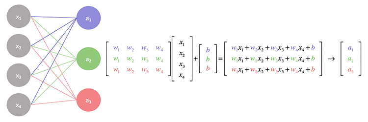
Now we'll combine matrices and vectors. Matrix-vector multiplication is the operation used to apply a linear transformation to a vector. This is precisely what happens when you pass data through a layer of a neural network.

The rule for multiplying a matrix $A$ by a vector $x$ is that each element of the resulting vector is the dot product of a row of the matrix $A$ with the vector $x$ .

Matrix-Vector Multiplication Illustration — This image illustrates the process. To get the first element of the output vector $A\mathbf{x}$, you take the dot product of the first row of $A$ with the vector $\mathbf{x}$. You repeat this for all rows of $A$.

Dimensionality Rule: For this to work, the number of columns in the matrix must equal the number of elements (rows) in the vector.
If $A$ is an m x n matrix and $x$ is an n x 1 vector, the result will be an m x 1 vector.

Let's watch a step-by-step example performed by hand.

Matrix Multiplication — Topic 19 of Machine Learning Foundations

The video 'Matrix Multiplication' by Jon Krohn gives a very clear, color-coded walkthrough of a matrix-vector multiplication.

Watch from 03:01 to 04:53. Follow the calculation for each element of the resulting vector. This visual breakdown makes the 'row-times-column' dot product rule very tangible.

This operation is at the heart of many ML models. For example, in a neural network, the matrix contains the "weights" of the connections, and the vector contains the input values. The multiplication calculates the weighted sum of inputs for each neuron in the next layer.

Matrix Multiplication and Vector Addition in a Neural Network — This diagram shows exactly how matrix-vector multiplication is used in a neural network. The weight matrix `W` transforms the input vector `X` into the pre-activation output vector `a`. The bias vector `b` is then added.

Matrix-Matrix Multiplication

The final step is multiplying two matrices together. You can think of this as performing several matrix-vector multiplications in parallel.

Mechanics: The element at row i, column j of the resulting matrix is the dot product of row i of the first matrix and column j of the second matrix.

Let's ground this with a clear, step-by-step textual guide.

Dot Product of a Matrix: Explained

The article 'Dot Product of a Matrix: Explained' on Built In breaks down a 2x2 matrix multiplication into four simple dot product calculations.

Read the sections 'How to Calculate the Dot Product of Two Matrices' and 'Tips for Calculating Dot Product of a Matrix'. Follow the four steps to see how each element of the final matrix is computed. Pay close attention to the rule for matching dimensions.

Dimensionality Rule: To multiply matrix $A$ by matrix $B$ (i.e., $A \times B$ ), the number of columns in $A$ must equal the number of rows in $B$ .
If $A$ is m x n and $B$ is n x p, the resulting matrix will be m x p.

Important Property: Matrix multiplication is not commutative. In general, $A \times B \neq = B \times A$ . The order matters!

Test your understanding!

Given the following matrix $A$ and vector $x$ :

A = [132004], x = 512

Check if the dimensions are compatible for the operation $A x$ .
Calculate the resulting vector $A x$ .

Show answer

Dimension Check: Matrix $A$ is 2 x 3 (2 rows, 3 columns). Vector $x$ is 3 x 1 (3 rows, 1 column). The inner dimensions match (3 and 3), so the multiplication is possible. The resulting vector will have dimensions 2 x 1.
Calculation:
- The first element of the result is the dot product of the first row of $A$ and $x$ :
  $(1 \times 5) + (2 \times 1) + (0 \times 2) = 5 + 2 + 0 = 7$
- The second element of the result is the dot product of the second row of $A$ and $x$ :
  $(3 \times 5) + (0 \times 1) + (4 \times 2) = 15 + 0 + 8 = 23$
So, the resulting vector is:
$A x = [723]$

From Math to Code: `inner` vs. `matmul`

Your goal is to understand the "why" behind the code you see or generate. In libraries like PyTorch and NumPy, these mathematical operations are implemented as single functions. A crucial distinction for practical use is understanding when to use a function for "similarity" versus "transformation".

The article Why Deep Learning Loves the Dot Product... which you read earlier has an excellent summary of this.

Why Deep Learning Loves the Dot Product and Matrix ...

Let's revisit 'Why Deep Learning Loves the Dot Product...' to see how these operations map to PyTorch functions.

Read the sections 'Pytorch Implementation' and 'In Summary'. Notice the difference between torch.inner() and torch.matmul(). This is a key practical takeaway for writing and understanding ML code.

In short:

Use np.inner or torch.inner when you want to compute similarity scores (dot products), like in attention mechanisms.
Use np.dot, @ operator, or torch.matmul when you want to perform linear transformations (matrix multiplication), like in the layers of a neural network.

Conclusion

In this lesson, we established the fundamental operational toolkit of linear algebra, which is the language of modern data science and machine learning.

Here are the key takeaways:

Vector and Matrix Operations are the computational core of ML.
The Dot Product takes two vectors and produces a scalar that measures their alignment or similarity.
Matrix-Vector Multiplication applies a linear transformation to a vector, which is how data is processed in models like linear regression and neural networks.
Matrix-Matrix Multiplication can be seen as applying a transformation to a whole set of vectors at once.
Dimensionality rules are critical: for any multiplication, the "inner" dimensions must match.
In code, it's important to distinguish between operations for similarity (inner) and for transformation (matmul).

In our next lesson, we will delve deeper into the properties of matrices by exploring eigenvalues and eigenvectors. These concepts will reveal how we can use matrix operations to understand the underlying structure and principal axes of variation within our data, a key idea behind dimensionality reduction techniques like PCA.

Recommended resources