Derivatives: Rates of Change and Optimization

From Slope to Instantaneous Change

You know that the slope of a straight line measures its steepness—how much the y value changes for a given change in the x value (often called "rise over run"). For a straight line, this rate of change is constant. But what about a curve, where the steepness is continuously changing? How can we talk about the "slope" at a single point on a curve?

This is the central question that derivatives answer. The derivative of a function at a specific point gives us the instantaneous rate of change at that very point. Geometrically, this is the slope of a straight line that just touches the curve at that point without crossing it—the tangent line.

To build this intuition visually, let's watch the first part of the following video. It does an excellent job of starting with the basic idea of slope and extending it to curves.

A Physical Analogy: Position, Velocity, and Acceleration

Given your engineering background, a physical analogy might make the idea of a derivative as a rate of change even more concrete. Think about a moving car:

• Its position can be described by a function of time, let's say $p(t)$.
• Its velocity is the rate of change of its position with respect to time. This is the first derivative of the position function, $v(t)=p^{\prime }(t)$.
• Its acceleration is the rate of change of its velocity. This is the first derivative of the velocity function, which also makes it the second derivative of the position function, $a(t)=v^{\prime }(t)=p^{\prime \prime }(t)$.

This article provides an excellent walkthrough of this exact example.

This relationship is key: the derivative function's value at any point tells you the slope, or rate of change, of the original function at that point.

Finding the "Best": How Derivatives Power Optimization

Now for the crucial link to machine learning. Why is finding the rate of change so important?

In many machine learning tasks, we define a loss function (also called a cost or error function). This function measures how "bad" our model's predictions are compared to the actual data. A high loss means bad predictions; a low loss means good predictions. The goal of training is to find the model parameters that make the loss as small as possible—that is, to find the minimum of the loss function.

Imagine the loss function as a landscape of hills and valleys. We want to find the bottom of the lowest valley.

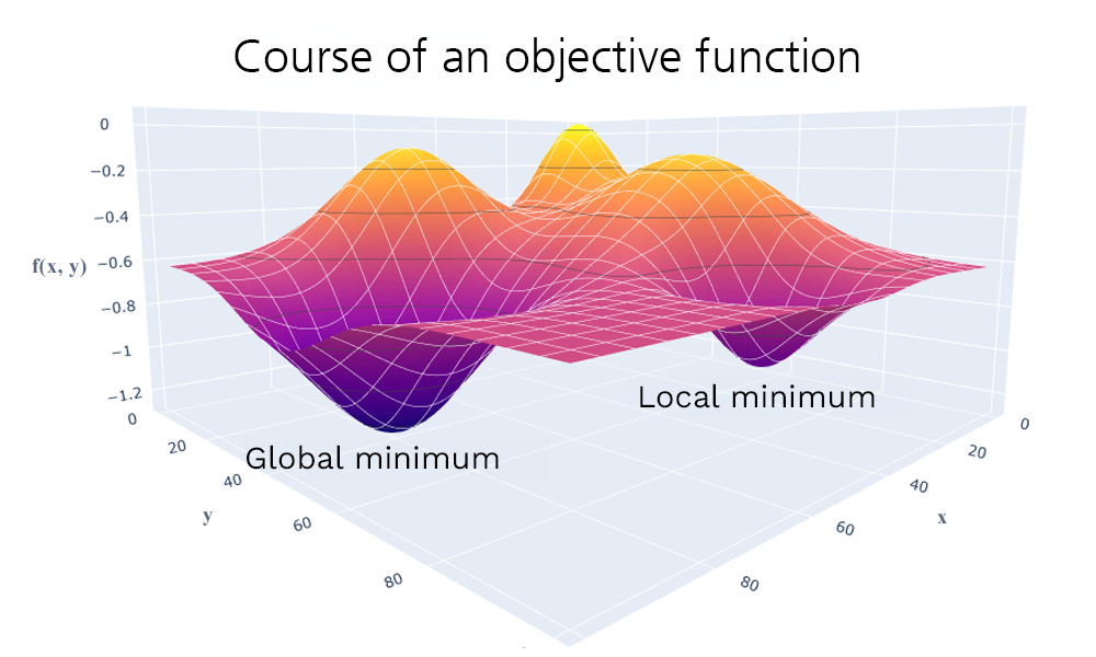
So, how do we find these low points? Think about what's special about the very bottom of a valley (a minimum) or the very top of a hill (a maximum). At these exact points, the ground is momentarily flat. The slope is zero.

This is the fundamental insight: To find the minima or maxima of a function, we can look for the points where its derivative is equal to zero.

The final part of the video you watched earlier explains this application in a machine learning context.

The Process: Finding Critical Points

Let's formalize this process, often called the First Derivative Test.

1. Define the function $f(x)$ you want to minimize or maximize.
2. Find its derivative, $f^{\prime }(x)$. To do this practically, we use differentiation rules. The most common one is the power rule, which states that if $f(x)=a{x}^n$, then its derivative is $f^{\prime }(x)=n\cdot a{x}^{n-1}$.
3. Find the critical points by setting the derivative to zero, $f^{\prime }(x)=0$, and solving for $x$.
4. Analyze the critical points. A critical point can be a minimum, a maximum, or neither (like a flat plateau, known as a saddle point). To tell the difference, we check the sign of the derivative on either side of the critical point:
   • If the derivative (slope) changes from negative to positive, the function goes from decreasing to increasing. This is a local minimum (a valley).
   • If the derivative (slope) changes from positive to negative, the function goes from increasing to decreasing. This is a local maximum (a hill).

This article provides a clear, step-by-step worked example of this process.

Conclusion

Congratulations on completing your first lesson! You've taken a significant first step into the mathematical engine that drives machine learning.

Here are the key takeaways:

• A derivative measures the instantaneous rate of change of a function, which is visually represented as the slope of the tangent line at a point.
• In machine learning, we aim to minimize a loss function to find the best model parameters. This process is called optimization.
• We can find potential minimum or maximum points (called critical points) by finding where the function's derivative is equal to zero.
• The First Derivative Test helps us confirm if a critical point is a minimum or maximum by checking the sign of the derivative on either side of it.

In this lesson, we focused on functions with a single variable. However, real-world machine learning models have thousands, millions, or even billions of parameters! In our next lesson, we will explore how the concept of a derivative extends to functions with many variables. This will lead us to the idea of the gradient, a crucial tool for optimizing the complex models you'll encounter in AI.