Bayesian Linear Regression

Hello! Welcome to the sixth lesson in our module on Bayesian methods.

In our previous lesson, we learned how to summarize a posterior distribution using a credible interval. This gave us an intuitive way to express our uncertainty about a parameter, stating directly "there is a 95% probability the true value lies in this range."

Today, we're going to apply this entire Bayesian framework to a model you're already familiar with from a frequentist perspective: linear regression. Our learning outcome is to apply Bayesian inference to a linear regression model. Instead of finding single "best-fit" coefficients, you will learn how to derive entire probability distributions for them, giving you a much richer understanding of your model's uncertainty. This lesson will also reveal a deep and surprising connection between the Bayesian approach and the regularization techniques you've already studied.

1. From Fixed Lines to Distributions of Lines

In standard (frequentist) linear regression, the goal is to find the single best-fit line that minimizes the sum of squared errors. This gives you one value for the intercept ( $β_{0}$ ) and one value for each slope ( $β_{j}$ ).

Bayesian Linear Regression with Uncertainty — This image illustrates the core idea of Bayesian linear regression. Instead of a single best-fit line (the orange line), we get a probability distribution of plausible lines, represented by the shaded orange region (the credible interval for our predictions).

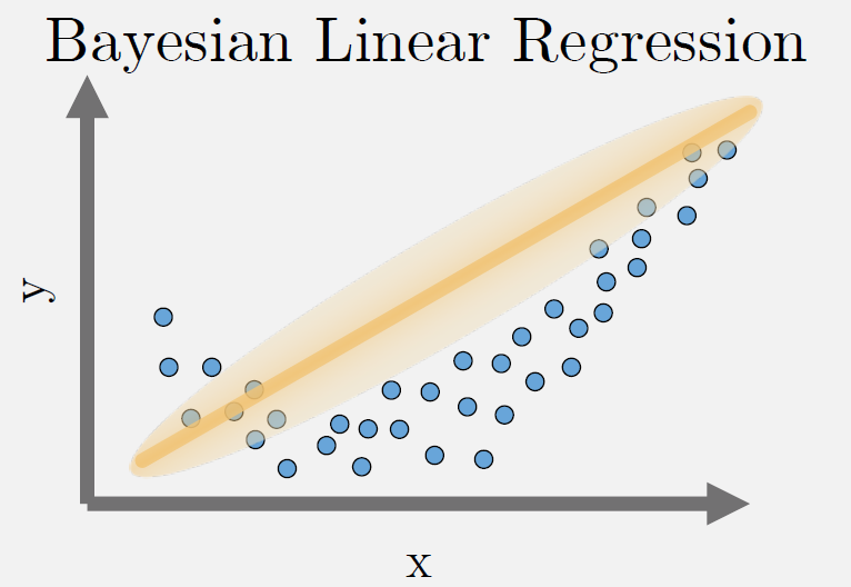
Bayesian linear regression reframes the problem. It asks: "Given the data, what is the entire probability distribution of plausible parameters?" The result is not a single value for each coefficient, but a full posterior distribution that tells us the mean, the credible interval, and our complete state of uncertainty about that parameter.

2. The Bayesian Framework for Linear Regression

To build a Bayesian model, we need to specify two key components from Bayes' theorem: the likelihood and the prior.

Posterior p (β ∣ Data) \propto Likelihood p (Data ∣ β) \times Prior p (β)

Let's see how this applies to linear regression.

a) The Likelihood: A Probabilistic View of Errors

The standard linear regression model is:

y = X β + ϵ

where we assume the errors $ϵ$ are independent and normally distributed with a mean of 0 and some variance $σ^{2}$ . This assumption is equivalent to defining our likelihood function. The likelihood, $p (y ∣ X, β, σ)$ , is a Gaussian distribution centered around the regression line:

p (y ∣ X, β, σ) = N (X β, σ^{2} I)

This simply states that for a given set of coefficients $β$ , the observed data $y$ is most likely to be close to the predicted values $X β$ , with deviations that follow a normal distribution.

b) The Prior: Encoding Our Beliefs about the Coefficients

Now for the Bayesian step: we must place a prior distribution on our parameters. We need priors for the coefficients $β$ and the error term's standard deviation $σ$ . Let's focus on $β$ .

A common and intuitive choice for the prior on $β$ is a Gaussian distribution centered at zero:

p (β) = N (0, τ^{2} I)

This prior encodes a belief that, before seeing any data, the coefficients are more likely to be small and close to zero. A large variance $τ^{2}$ makes this a "weakly informative" prior, meaning we don't have a strong initial opinion.

c) The Posterior: Combining Priors and Data

Once we have the likelihood and the prior, we use Bayes' theorem to find the posterior distribution of the coefficients, $p (β ∣ y, X)$ . This posterior distribution represents our updated belief about the coefficients after observing the data.

When we use a Gaussian likelihood and a Gaussian prior, the resulting posterior is also a Gaussian distribution. This special case is known as using a conjugate prior, which simplifies the math. However, the real magic lies in the connection this framework has to a concept you already know: regularization.

3. The "Aha!" Moment: Priors are Regularization

You've learned about Ridge (L2) and Lasso (L1) regularization as methods to prevent overfitting by adding a penalty term to the cost function. Have you ever wondered where those penalty terms come from? Bayesian inference provides the answer.

Let's watch a video that connects these dots.

Bayesian Linear Regression : Data Science Concepts

The following video from the 'ritvikmath' channel does an excellent job of explaining how the Bayesian approach to linear regression naturally leads to the same optimization problem as Ridge and Lasso regression.

Watch the video from the beginning to 04:50, and then from 09:30 to 13:40. Focus on these key points: The review of why regularization is needed (to control high variance in OLS solutions). The setup of the Bayesian problem: maximizing the posterior probability, which is proportional to likelihood * prior. The crucial reveal: How choosing a Gaussian prior for the beta coefficients leads exactly to the Ridge (L2) regression cost function. How choosing a Laplacian prior leads to the Lasso (L1) regression cost function.

As the video explains, finding the Maximum A Posteriori (MAP) estimate—the mode (peak) of the posterior distribution—is equivalent to minimizing a regularized loss function.

Gaussian Prior on $β$ $⟹$ Ridge (L2) Regularization
Laplacian Prior on $β$ $⟹$ Lasso (L1) Regularization

This is a profound insight. Regularization is not just an ad-hoc trick; it is the direct consequence of expressing a prior belief that model coefficients should be small. The regularization parameter $λ$ is directly related to the variance of our prior ( $τ^{2}$ ) and the variance of our data ( $σ^{2}$ ). A stronger prior belief (smaller $τ^{2}$ ) corresponds to stronger regularization (larger $λ$ ).

Test your understanding!

A colleague is training a linear regression model and finds that the coefficients are very large, leading to overfitting. They decide to add L2 regularization to "shrink the coefficients." Based on what you just learned, how could you reframe their action from a Bayesian perspective?

Show answer

You could explain that adding L2 regularization is equivalent to moving from a simple Maximum Likelihood Estimation (which has no prior) to a Maximum A Posteriori (MAP) estimation. By adding the L2 penalty, they are implicitly placing a Gaussian prior on the model's coefficients. This prior encodes a belief that smaller coefficients are more probable than larger ones, which serves to "shrink" them towards zero and combat overfitting.

4. Bayesian Linear Regression in Practice with PyMC

While finding the MAP estimate is useful, the full power of Bayesian inference comes from finding the entire posterior distribution. For complex models, calculating this distribution by hand is difficult or impossible. This is where probabilistic programming languages (PPLs) like PyMC are essential. They use numerical methods like Markov Chain Monte Carlo (MCMC) to draw samples from the posterior distribution for us.

Let's see how this is done.

Gentle introduction of Bayesian Linear Regression

This article, 'Gentle introduction of Bayesian Linear Regression', provides a great overview and a clear PyMC code example.

Please read section 3, 'PyMC implementation using real-world dataset'. Focus on the code block where the PyMC model is defined. Notice how each line of code corresponds directly to the statistical concepts we've discussed: pm.HalfNormal("sigma", ...) defines the prior for the error term. pm.Normal("beta", ...) defines the Gaussian prior for the regression coefficients. pm.Normal("y_hat", mu=mu, ...) defines the likelihood, linking the parameters to the observed data.

The process shown in the article is the standard workflow:

Define Priors: Specify prior distributions for all unknown parameters (sigma, beta, beta0).
Define the Likelihood: Define the model that connects the parameters to the data (mu = beta0 + at.dot(X_train, beta) and y_hat).
Sample from the Posterior: Use a function like pm.sample() to run the MCMC sampler.

The output isn't a single number for each coefficient, but thousands of samples that form a picture of the posterior distribution.

Interpreting the Results

Once we have these samples, we can analyze them to understand our model.

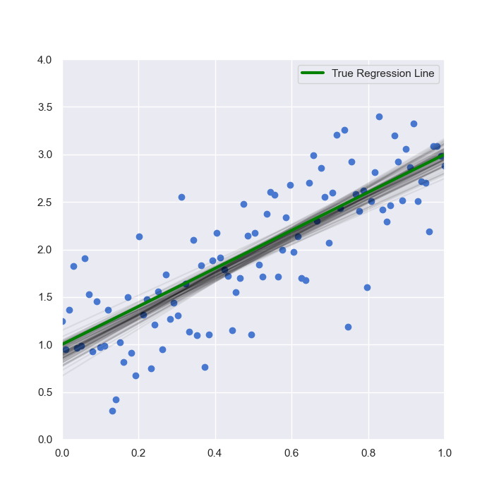
Bayesian Linear Regression with Posterior Samples — This image visualizes the posterior samples. The green line is the (unknown) true regression line. The faint grey lines are individual regression lines, each created using a set of coefficient samples from our posterior distribution. The density of these lines shows us where the model is most certain.

From these posterior samples, we can:

Plot the distributions for each coefficient to see its shape, mean, and spread.
Calculate a mean for each coefficient, which serves as a robust point estimate.
Calculate a 95% credible interval for each coefficient, giving us a range of plausible values. For example, if the 95% credible interval for a coefficient beta_1 is [2.1, 3.5], we can say there is a 95% probability that the true value of beta_1 lies in this range. If the interval contains zero (e.g., [-0.5, 1.2]), it suggests the variable may not have a statistically significant effect.

This provides a much more complete picture of model uncertainty than a single p-value from a frequentist regression.

Conclusion

In this lesson, you've taken a significant step in applying Bayesian methods to a practical machine learning model. You've seen that Bayesian linear regression isn't just a different technique; it's a paradigm shift that moves from seeking single best-fit parameters to characterizing our full uncertainty about them.

Key Takeaways:

Bayesian linear regression models parameters (coefficients) as probability distributions rather than fixed point estimates.
The framework consists of defining a likelihood (probabilistic model of the data) and priors (our initial beliefs about the parameters).
The choice of prior is deeply connected to regularization: a Gaussian prior on coefficients is equivalent to L2 (Ridge) regularization, providing a theoretical justification for it.
The output is a posterior distribution for each parameter, which we can summarize with means and credible intervals to quantify our uncertainty.
Probabilistic programming libraries like PyMC automate the difficult process of finding the posterior distribution.

Preview of the Next Lesson:

We briefly touched upon the idea of Maximum A Posteriori (MAP) estimation—finding the peak of the posterior distribution. In our next lesson, we will explore this concept in more detail. You'll learn how MAP provides a bridge between full Bayesian inference and simpler point estimation, offering a practical optimization target that incorporates prior knowledge.

Recommended resources