Bayesian Credible Intervals vs. Frequentist Confidence Intervals

Hello! Welcome to the fifth lesson in our module on Bayesian methods.

In our last lesson, we focused on the mechanics of Bayesian updating, learning how to compute a full posterior distribution, like Beta(50, 550), by combining a prior with new data. While the posterior distribution contains everything we know about a parameter, it's often too detailed to communicate easily. We need a concise summary.

Today, we'll learn how to create and use one of the most important summaries in Bayesian analysis. Our learning outcome is to construct and interpret Bayesian credible intervals and compare them to frequentist confidence intervals. You'll discover that credible intervals provide an intuitive way to express uncertainty that aligns directly with how we naturally think about probability.

1. The Core Philosophical Divide: A Quick Refresher

Before diving into the intervals themselves, it's crucial to recall the fundamental difference between the frequentist and Bayesian views of probability. This difference is the root cause of why their intervals are interpreted so differently.

Bayesian vs. Frequentist Statistics ... MADE EASY!!!

Let's watch a short segment from the 'Stats with Brian' channel that perfectly illustrates this philosophical split and how it leads to different interval interpretations.

Watch the video from 00:12 to 04:25. Pay close attention to: The definition of probability for each school of thought: long-run frequency (frequentist) vs. degree of belief (Bayesian). The thought experiment about the 'government agent'. It's a fantastic illustration of why the interpretation of a frequentist confidence interval is so specific and counter-intuitive.

This video highlights the core distinction:

Frequentist: A parameter (like the true average height of a population) is a single, fixed, unknown constant. Our data is random. Probability is about the long-run performance of our methods over many hypothetical repeated experiments.
Bayesian: A parameter is a random variable that we are uncertain about. We can express this uncertainty using probability. Our data is fixed (it's what we observed). Probability is about our degree of belief in the parameter's value.

This philosophical split directly impacts how we define and talk about uncertainty intervals.

2. The Frequentist Confidence Interval: A Review

From your basic statistics knowledge, you're familiar with the 95% confidence interval. Let's formalize its interpretation.

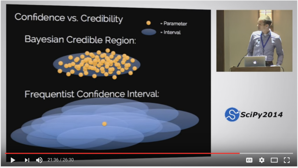
A frequentist confidence interval is like a net. Imagine the true parameter is a stationary fish in a lake. Each time you take a sample and calculate an interval, you are throwing a net. Some of your nets will catch the fish, and some will miss.

A 95% confidence interval is a range constructed by a procedure that, if repeated infinitely, would produce nets that "capture" the true, fixed parameter 95% of the time.

Bayesian Credible Region vs. Frequentist Confidence Interval — This image visually contrasts the two approaches. On the right, the frequentist view: the orange dot (the parameter) is fixed, while the blue ellipses (the intervals) are random and vary with each sample. We hope our particular interval is one of the ones that contains the dot.

Therefore, the correct interpretation is:

"We are 95% confident that the procedure used to generate this interval captures the true population parameter."

It is incorrect to say:

"There is a 95% probability that the true parameter lies within this specific interval."

As the video showed, once the interval is calculated (e.g., 64-68 inches) and the true value is revealed (e.g., 63 inches), the probability of the true value being in that interval is either 0% or 100%. The "95%" refers to the success rate of the method, not the probability associated with a single outcome.

3. The Bayesian Credible Interval: An Intuitive Alternative

The Bayesian approach provides an interval that aligns with the interpretation everyone wants to use for a confidence interval.

A credible interval is a range of values where we believe the true parameter lies with a certain probability, given our evidence. It's a direct statement about the parameter's plausible values.

Referring back to the image Bayesian Credible vs Frequentist Confidence Intervals, the left side illustrates the Bayesian view: the blue ellipse (the interval) is a fixed summary of our posterior belief, and the orange dots represent the plausible values the parameter could take, with most of their mass falling inside the interval.

The interpretation is direct and intuitive:

"Given our data, there is a 95% probability that the true parameter lies within this interval."

This statement is possible because in the Bayesian world, the parameter itself is a random variable, and the posterior distribution we calculated in the last lesson, e.g., Beta(50, 550), describes our belief about its possible values.

4. Constructing a Credible Interval

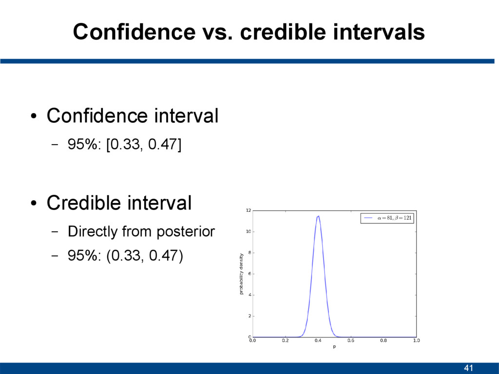
So, how do we get this interval from the posterior distribution? A 95% credible interval is simply a range that contains 95% of the area under the posterior probability density curve.

Confidence vs. Credible Intervals Comparison — This image connects the posterior distribution to the credible interval. The curve is the posterior probability density (in this case, a Beta(81, 121) distribution). The 95% credible interval [0.33, 0.47] is the range on the x-axis that contains 95% of the area under that curve.

The most common method to construct this is the Equal-Tailed Interval:

Find the value L such that 2.5% of the posterior probability is below it.
Find the value U such that 2.5% of the posterior probability is above it (or 97.5% is below it).
The 95% credible interval is [L, U].

Let's use the example from our last lesson's exercise. We had a Beta(5, 95) prior and observed 45 successes in 500 trials, resulting in a Beta(50, 550) posterior.

To find the 95% credible interval, we need to find the 2.5th and 97.5th percentiles of this distribution. We can do this easily with statistical software. For example, in Python:

from scipy.stats import beta

alpha_post = 50
beta_post = 550

# Find the 2.5th and 97.5th percentiles
lower_bound = beta.ppf(0.025, alpha_post, beta_post)
upper_bound = beta.ppf(0.0975, alpha_post, beta_post) # Typo in original. Should be 0.975

# Correcting the upper bound calculation
upper_bound = beta.ppf(0.975, alpha_post, beta_post)

print(f"95% Credible Interval: [{lower_bound:.3f}, {upper_bound:.3f}]")
# Output: 95% Credible Interval: [0.066, 0.106]

Our 95% credible interval for the click-through rate is approximately [0.066, 0.106]. We can state that, given our prior and the A/B test data, there is a 95% probability that the true click-through rate is between 6.6% and 10.6%.

5. Head-to-Head Comparison

Let's consolidate the differences in a clear table, adapted from the "Program Evaluation" resource.

Feature	Frequentist	Bayesian
Core Idea	$P (Data ∣ θ)$ Probability of seeing the data, given a hypothesis about the parameter $θ$ .	$P (θ ∣ Data)$ Probability of the parameter $θ$ , given the data.
Nature of $θ$	$θ$ is a fixed, unknown constant.	$θ$ is a random variable with a probability distribution.
Nature of Data	Data is a random sample; we can imagine repeating the experiment.	Data is fixed; it's what was observed.
Interval Name	Confidence Interval	Credible Interval
Interpretation	"There's a 95% probability that this range contains the true value of $θ$ ."	"There's a 95% probability that the true value of $θ$ falls in this range."
Governing Question	"How certain are we that the true parameter is not some null value (e.g., zero)?"	"Given our data and prior, what are the plausible values for the true parameter?"

Test your understanding!

Suppose you are analyzing the Milgram experiment from our last lesson, where your posterior for the proportion of people who obey authority was Beta(27, 24). You calculate an interval of [0.39, 0.65].

If this is a 95% credible interval, how would you interpret it in plain English?
If this were a 95% confidence interval, how would that interpretation be different?

Show answer

As a Credible Interval: "Based on the experiment's data and our prior beliefs, there is a 95% probability that the true proportion of people who would obey is between 39% and 65%." This is a direct statement of belief about the parameter's value.
As a Confidence Interval: "The procedure used to calculate the interval [0.39, 0.65] will, in 95% of repeated experiments, produce an interval that contains the true proportion of people who obey." You cannot say there is a 95% probability that the true proportion is in this specific interval. The confidence is in the method, not the result.

Conclusion

In this lesson, we explored one of the most practical and powerful tools in the Bayesian toolkit: the credible interval. You learned not just how to construct one from a posterior distribution, but also why its interpretation is so fundamentally different from its frequentist cousin, the confidence interval.

Key Takeaways:

The difference between credible and confidence intervals stems from the core philosophical disagreement between Bayesian (probability as belief) and Frequentist (probability as long-run frequency) statistics.
A confidence interval expresses our confidence in the procedure used to create the interval.
A credible interval expresses our belief about the parameter itself, providing a direct probabilistic range for its true value.
A credible interval is constructed by finding a range that contains a specified percentage (e.g., 95%) of the area under the posterior distribution curve.

Preview of the Next Lesson:

So far, we have assembled the key components of a Bayesian analysis: defining priors, computing the posterior, and summarizing it with a credible interval. In our next lesson, we will put all these pieces together and apply Bayesian inference to a linear regression model. This will be our first look at how the Bayesian approach can augment a standard machine learning model, providing richer insights than a frequentist analysis alone.