Introduction to MAP Estimation

1. The Problem with Relying Only on Data: A Limit of MLE

Let's start with a quick thought experiment. Imagine you're tasked with estimating the fairness of a coin. You flip it three times and, just by chance, you get heads every time.

If we use Maximum Likelihood Estimation (MLE), which we've seen before, we find the parameter (the probability of heads, $\theta$) that makes our observed data most likely. In this case, the MLE for $\theta$ would be 1.0. This estimate implies that the coin will always land on heads, which seems like a very strong and probably incorrect conclusion based on only three flips.

This simple example highlights a key weakness of MLE: it can be overly sensitive to small or unrepresentative datasets because it has no mechanism to incorporate our common-sense knowledge. This is where MAP estimation comes in.

To see a great explanation of this problem, let's watch the beginning of the following video.

As the video explains, the solution is to use a Bayesian approach to incorporate our prior knowledge—for example, our belief that most coins are reasonably fair.

2. Combining Beliefs and Data: The Heart of MAP

MAP estimation formalizes this process using Bayes' theorem. Recall the theorem, which provides a way to update our beliefs in light of new evidence:

• Likelihood $P(\text{Data}|\theta )$: The same term used in MLE. It asks: "What is the probability of seeing this data, given a specific parameter value $\theta$?"
• Prior $P(\theta )$: This is new. It represents our belief about the parameter $\theta$ before seeing any data. For the coin, our prior might be a probability distribution peaked around $\theta =0.5$.
• Posterior $P(\theta |\text{Data})$: Our updated belief about $\theta$ after combining the data and our prior.

While full Bayesian inference (like we saw in the last lesson) is concerned with the entire posterior distribution, MAP estimation simply seeks the single most probable parameter value, i.e., the peak or mode of the posterior distribution.

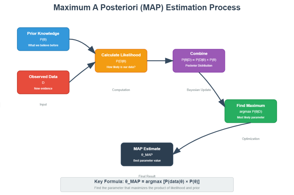
The goal of MAP is to find the $\theta$ that maximizes the posterior probability:

Notice that when we are looking for the value of $\theta$ that maximizes this expression, the denominator $P(\text{Data})$ is constant with respect to $\theta$. Therefore, we can ignore it for optimization purposes. This simplifies our goal to:

In plain English, the MAP estimate is the parameter value $\theta$ that maximizes the product of the likelihood and the prior.

This flow diagram provides a great visual summary of the process.

3. MAP in Action: Revisiting the Coin Flip

Let's make this concrete with an example. The following reading provides a fantastic, practical walkthrough.

Let's break down the key insight from that example, where we observe 7 heads in 10 flips.

• The Likelihood function, based purely on the data (7 heads, 3 tails), peaks at the MLE estimate: $\theta =0.7$.
• Our Prior belief is that the coin is probably fair. We can represent this with a Beta distribution that peaks at $\theta =0.5$.
• The Posterior distribution is the result of multiplying the likelihood and the prior. Its peak is a compromise between the two.

An Intuitive View: "Imaginary Flips"

There's a beautifully simple way to think about how priors work in this context, which comes from Tom Mitchell's machine learning book. You can think of a prior as adding "imaginary" data to your observations.

For the coin-flipping problem, a common prior is the Beta distribution. For instance, choosing a Beta(2, 2) prior is mathematically equivalent to adding 1 imaginary head and 1 imaginary tail to our data before calculating the probability.

Let's see the math:

• MLE Estimate:
  ${\hat{\theta }}_{MLE}=\frac{{\alpha }_1}{{\alpha }_1+{\alpha }_0}=\frac{7}{7+3}=0.7$
  where ${\alpha }_1$ is the count of heads and ${\alpha }_0$ is the count of tails.

• MAP Estimate with a Beta(2, 2) prior:
  ${\hat{\theta }}_{MAP}=\frac{{\alpha }_1+{\gamma }_1}{{\alpha }_1+{\gamma }_1+{\alpha }_0+{\gamma }_0}=\frac{7+1}{7+1+3+1}=\frac{8}{12}\approx 0.667$
  where ${\gamma }_1=1$ and ${\gamma }_0=1$ are our imaginary heads and tails from the prior.

The MAP estimate is "pulled" away from the MLE of 0.7 towards our prior belief of 0.5. If we have very little data, the prior has a strong influence. If we have a lot of data, the influence of the few imaginary flips becomes negligible, and the MAP estimate will converge to the MLE estimate.

4. The Connection Between MAP and MLE

You might now be wondering about the relationship between these two estimation methods. As we've hinted, there's a direct link.

MLE is a special case of MAP estimation.

This occurs when we choose a uniform prior. A uniform prior means we believe all possible parameter values are equally likely before seeing the data (e.g., $P(\theta )=\text{constant}$). If $P(\theta )$ is a constant, then maximizing the product $P(\text{Data}|\theta )P(\theta )$ becomes equivalent to maximizing just the likelihood $P(\text{Data}|\theta )$.

So, performing MLE is the same as performing MAP with the assumption of a completely uninformative prior. MAP generalizes this by allowing you to inject your domain knowledge into the estimation problem.

Conclusion

In this lesson, you've explored the core principles of Maximum A Posteriori estimation. It offers a pragmatic and powerful middle ground, blending the data-driven objectivity of MLE with the ability to incorporate prior beliefs from the Bayesian world.

Key Takeaways:

• MAP estimation finds the parameter value that maximizes the posterior probability, $P(\theta |\text{Data})$.
• It provides a balance between the evidence from the data (likelihood) and our initial beliefs (prior). The mathematical formulation is ${\theta }_{\text{MAP}}=\underset{\theta }{\mathrm{argmax}}P(\text{Data}|\theta )P(\theta )$.
• MAP acts as a form of regularization, preventing the extreme estimates that MLE can produce with limited data by "pulling" the estimate toward the prior.
• MLE is a special case of MAP where the prior distribution is uniform (i.e., we assume no prior knowledge).

Preview of the Next Lesson:

This lesson concludes our module on Bayesian methods! As we move into the next module, Optimization for Machine Learning, we will start by formally defining the role of a loss function. You are now perfectly equipped to understand a deep connection: the MAP estimation objective is often equivalent to minimizing a loss function.

For example, maximizing $P(\text{Data}|\theta )P(\theta )$ is the same as minimizing $-\log (P(\text{Data}|\theta ))-\log (P(\theta ))$. This expression is precisely a loss function composed of a data-fit term (the negative log-likelihood) and a regularization term (the negative log-prior). We will explore this powerful idea as we begin our journey into optimization.