Gradient Descent for Model Optimization

Hello! Welcome to the third lesson in our module on Optimization for Machine Learning.

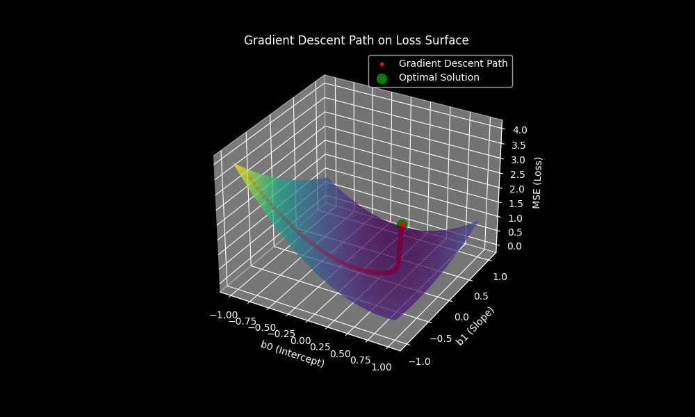
In the last lesson, we described gradient descent as an iterative algorithm. We established that it's like a hiker trying to find the bottom of a valley in a thick fog. The hiker's only information is the steepness of the ground right under their feet (the gradient). By repeatedly taking small steps in the steepest downhill direction, they eventually reach the valley floor.

Today, we're moving from this conceptual understanding to practical application. Our goal is to implement gradient descent to optimize the parameters of a simple model. We will translate the update rule we learned, $w_{new} = w_{old} - α \cdot \nabla J (w_{old})$ , into working Python code. This will solidify your understanding of how a model truly "learns" from data.

Visualizing the Process in Code

Before we write the code ourselves, let's watch a dynamic visualization of what we're about to build. This will help connect the abstract idea of a "ball rolling downhill" to the iterative updates a computer performs.

Gradient Descent From Scratch in Python - Visual Explanation

The video 'Gradient Descent From Scratch in Python' from the NeuralNine channel provides an excellent animated view of the process for a simple function. It shows exactly how the parameter is updated in each iteration.

Please watch from 4:59 to 13:19. You don't need to follow every line of code just yet. Instead, focus on: How the red dot (the current parameter value) iteratively moves down the curve. The code that implements the core update rule: new_x = current_pos - learning_rate * derivative. The visual effect of the ball 'rolling' down the hill towards the minimum.

This animation is the heart of what we will implement. The computer doesn't "see" the whole curve; at each step, it just calculates the slope (derivative) and takes a small step in the opposite direction.

Implementing Gradient Descent for Linear Regression

Now, let's apply this to a concrete machine learning model: simple linear regression. As a refresher, our model's goal is to find the best-fit line for our data.

Model: The equation for the line is $y_{predicted} = m x + b$ , where $m$ is the slope and $b$ is the intercept. These are the two parameters we need to optimize.
Loss Function: We'll use the Mean Squared Error (MSE), which measures the average squared difference between the actual $y$ values and our predicted $y$ values. $J (m, b) = \frac{1}{n} i = 1 \sum n (y_{i} - (m x_{i} + b))^{2}$
Gradient: To use gradient descent, we need the partial derivatives of the loss function with respect to each parameter, $m$ and $b$ . As a reminder from your calculus background, a partial derivative tells us how the loss function changes if we nudge just one parameter, keeping the others fixed. Without going through the full derivation, the gradients are: $\frac{\partial J}{\partial m} = - \frac{2}{n} i = 1 \sum n x_{i} (y_{i} - y_{predicted})$ $\frac{\partial J}{\partial b} = - \frac{2}{n} i = 1 \sum n (y_{i} - y_{predicted})$

These formulas give us the direction of steepest ascent. Now we have all the pieces to build our algorithm.

Step-by-Step Python Implementation

We will now walk through a complete implementation from scratch. The following video is a fantastic resource that builds the code line by line, explaining each step clearly.

Machine Learning Tutorial Python - 4: Gradient Descent and Cost Function

This video from the codebasics channel will guide us through implementing gradient descent for linear regression in Python. We'll start with the theory and then translate it directly into code.

First, watch from the beginning to 16:04. This covers the core logic. 0:00 - 5:05: A quick recap of the goal (finding the best-fit line) and the MSE cost function. 5:05 - 10:10: The intuition of taking 'baby steps' down the cost function surface, guided by the slope. 10:10 - 16:04: An explanation of the derivatives and the final update equations we'll use.

Now that you have the theoretical setup, let's see it translated into code.

Machine Learning Tutorial Python - 4: Gradient Descent and Cost Function

Continuing with the same video, let's watch the coding part. Pay close attention to how the formulas for the derivatives are converted into NumPy operations.

Watch from 16:04 to 21:41. Follow along with the code structure: Initialize m_current and b_current (usually to 0). Define hyperparameters: iterations and learning_rate. Start a for loop that runs for the number of iterations. Inside the loop, calculate y_predicted. Calculate the derivatives md and bd using the formulas. Update m_current and b_current using the learning rate and the derivatives.

This implementation directly mirrors the algorithm: initialize, then loop to calculate gradients and update parameters.

Tuning the Learning Rate

In the previous lesson and the videos you just watched, the learning rate ( $α$ ) was mentioned as a critical hyperparameter. It controls how big of a step we take downhill.

Too small: The algorithm will be very slow to converge.
Too large: The algorithm can overshoot the minimum and bounce around chaotically, failing to converge at all. It might even diverge, with the cost getting larger and larger.

Finding a good learning rate is often a process of trial and error. A key part of implementing gradient descent is monitoring the cost at each iteration to ensure it's consistently decreasing.

Let's see a practical demonstration of tuning this value.

Machine Learning Tutorial Python - 4: Gradient Descent and Cost Function

Let's return to the codebasics video to see how to monitor the cost and adjust the learning rate.

Watch the final part, from 21:41 to 26:43. Notice how the author: Adds a calculation for the cost inside the loop and prints it. Experiments with a higher learning rate, which causes the cost to increase (divergence). Finds a 'sweet spot' for the learning rate that decreases the cost effectively.

Gradient Descent Path on Loss Surface — This visualization shows a successful gradient descent path on a 3D loss surface. A well-tuned learning rate ensures the path moves smoothly downhill towards the optimal solution (green dot). If the learning rate were too high, this path might zigzag wildly across the valley or even shoot up the other side.

Test your understanding!

You are training a model using gradient descent and you plot the cost function at each iteration. You notice that the cost is oscillating wildly and sometimes increasing. What is the most likely cause of this behavior, and what is the first thing you should try to fix it?

Show answer

The most likely cause is that the learning rate is too high. This is causing the algorithm to overshoot the minimum of the cost function at each step.

The first thing you should do is reduce the learning rate (e.g., by a factor of 10, from 0.01 to 0.001) and run the training again to see if the cost starts to decrease steadily.

A More Professional Implementation

The implementation in the video is excellent for learning because it's very explicit. However, in practice, we often use vectorized operations for efficiency, which is a strength of libraries like NumPy. This avoids explicit for loops over data points.

The following resource shows a more standard, vectorized implementation of the same algorithm.

Implementing Gradient Descent in Python

The article 'Mastering Gradient Descent' provides a slightly more advanced and efficient implementation using NumPy's capabilities. This style is closer to what you'd see in real-world ML codebases.

Read the sections 'Machine Learning Use Case: Linear Regression' and 'Implementing Gradient Descent in Python'. Compare the provided Python code block with the one from the video. Notice how it uses X.dot(theta) for prediction and X.T.dot(errors) to calculate gradients without an explicit loop. This is a more efficient, vectorized approach.

This more compact style is something you will encounter frequently. The underlying logic is identical to what we built step-by-step; it's just expressed more concisely using matrix and vector operations. This is a common pattern in your engineering field, where leveraging optimized libraries like NumPy is preferred over manual loops for performance.

Conclusion

In this lesson, you have successfully bridged the gap between the theory of gradient descent and its practical implementation. You took the abstract concept of "moving downhill" and turned it into a concrete Python algorithm that can find the optimal parameters for a linear regression model.

Key Takeaways:

Implementing gradient descent requires translating the mathematical components (model function, loss function, gradients) into code.
The core of the implementation is an iterative loop that calculates predictions, computes gradients, and updates parameters at each step.
Monitoring the cost function is crucial for debugging and for tuning the learning rate, which is arguably the most important hyperparameter in gradient descent.
Vectorized implementations (using matrix operations) are more efficient and common in practice than using explicit loops over the data.

Preview of the Next Lesson:

The algorithm we implemented is known as Batch Gradient Descent because it uses the entire batch of training data to calculate the gradient at every single step. For very large datasets, this can be computationally expensive. In our next lesson, we will explore more efficient variations: "Differentiate between batch, mini-batch, and stochastic gradient descent and their trade-offs."

Recommended resources

Visualizing the Process in Code

Implementing Gradient Descent for Linear Regression

Step-by-Step Python Implementation

Tuning the Learning Rate

A More Professional Implementation

Conclusion